Lecture 11: Algorithms and Their Characteristics - Simulation and Optimization: Lecture Notes

In Lectures 8 to 10 we modeled problems as (I)LO models and let a solver find the optimal solution. The solver runs an algorithm, such as the simplex method or branch and bound. This notebook explains what an algorithm is, how the algorithms in this lecture are written down, and how algorithms differ from each other. The next three notebooks each take one classical problem: Shortest Path, Maximum Flow and the Traveling Salesman Problem. Each defines the problem, gives an example, and solves it in two ways: with an (I)LO approach, a model solved with pulp, and with a dedicated algorithm. The dedicated algorithm is often the way to go in practice, because it is much faster. For the traveling salesman problem, however, no fast exact algorithm is known. The last notebook, Complexity and Heuristics, explains why some problems can be solved fast and others apparently cannot, and how heuristics find good solutions for the hard ones.

Learning outcomes

On completion of this notebook, you will be able to:

explain what an algorithm is and give examples;
read an algorithm written with a start step, a repeated step and a stopping rule, and say what each intermediate quantity means;
characterize an algorithm as dedicated or general, as polynomial or non-polynomial, and as exact or heuristic.

What Is an Algorithm?¶

An algorithm is a set of computer instructions that finds a solution for a problem. More precisely, it is a computational procedure that yields a solution for every problem in a class of problems: not for one specific instance, but for every instance of the same type. Examples we have already met or will meet in this lecture:

the simplex method solves LO problems;
the branch-and-bound method solves ILO problems (see Integer Optimization);
Dijkstra’s algorithm solves the shortest path problem (see Shortest Path).

How We Write Down an Algorithm¶

Most algorithms in this lecture improve something step by step: a distance estimate, a flow, a tour. To make clear what is going on halfway through, we first define the quantities the algorithm keeps track of and say exactly what they mean at every step. The algorithm itself then has three parts:

Start: give every quantity its initial value;
While some condition holds: the steps that are repeated, each one updating the quantities;
the stopping rule (the condition of the while loop fails) and what the quantities then give us.

A small example shows the style. We want the largest of $n$ numbers $a_1, a_2, \dots, a_n$ . Define, for $k = 1, \dots, n$ ,

m_k = \text{the largest of the first } k \text{ numbers } a_1, \dots, a_k.

(1)

Our aim is $m_n$ . The algorithm is:

Start: $k = 1$ and $m_1 = a_1$ .
While $k < n$ :
- $m_{k+1} = \max\{m_k, a_{k+1}\}$ ;
- $k = k + 1$ .

The update step is correct because of what $m_k$ means: the largest of the first $k + 1$ numbers is either the largest of the first $k$ numbers, or the new number $a_{k+1}$ . When the loop stops, $k = n$ and $m_n$ is the answer. In Python:

numbers = [4, 9, 2, 7, 11, 3]

largest = numbers[0]  # m_1
for a in numbers[1:]:
    largest = max(largest, a)  # m_{k+1} = max(m_k, a_{k+1})
print("largest number:", largest)

largest number: 11

The algorithm makes $n - 1$ comparisons, one per repetition of the loop, so its running time grows linearly with $n$ . Counting steps like this is the start of Complexity and Heuristics.

Each algorithm in this lecture also comes with Python code that follows its description line by line, as the code above does. You do not need to be able to program these algorithms from scratch. You should be able to read the code and follow what it does: which line carries out which step of the algorithm, and what each variable holds at every step. Running the code on a small example and comparing it with your own steps by hand is a good way to check that.

Characteristics of Algorithms¶

Algorithms can be characterized in three ways.

Dedicated or general. A dedicated algorithm solves one type of problem, such as Dijkstra’s algorithm for the shortest path problem or the Ford-Fulkerson algorithm for the maximum flow problem. A general algorithm solves a wide range of problems: the simplex method solves any LO problem, branch and bound any ILO problem, and evolutionary algorithms can be applied to almost any optimization problem. A dedicated algorithm uses the structure of its problem, which usually makes it much faster than solving an (I)LO model of the same problem with a general algorithm.
Polynomial or non-polynomial complexity. The complexity of an algorithm describes how its running time grows with the size of the problem, for example with the number of nodes $n$ of a network. If the running time grows like $n^2$ (polynomial), large instances are typically no problem; if it grows like $n!$ (non-polynomial), even moderate instances take forever. See Complexity and Heuristics.
Exact or heuristic. An exact algorithm is guaranteed to find an optimal solution. A heuristic is a best-effort method: a shortcut algorithm whose aim is not the optimal solution but a good solution in a reasonable amount of time. Training a neural network by gradient descent is an example: it finds good network weights, but nobody claims they are the best possible ones.

Why not just use the best general algorithm for everything? The no free lunch theorem (Wolpert & Macready, 1997) says that no such best algorithm exists: averaged over all possible problems, all search and optimization algorithms perform equally well. If an algorithm does better on one class of problems, it pays for that with worse performance on another class. Good performance comes from matching the algorithm to the structure of the problem, which is what dedicated algorithms do.

The table below characterizes the algorithms of Lectures 8 to 11. The running times are explained in the notebooks of the algorithms and in Complexity and Heuristics.

Table 1:Characteristics of the algorithms in Lectures 8 to 11.

algorithm	problem	dedicated or general	complexity	exact or heuristic
simplex method	LO	general	non-polynomial in the worst case, fast in practice	exact
branch and bound	ILO	general	non-polynomial	exact
Dijkstra’s algorithm	shortest path	dedicated	polynomial ( $n^2$ )	exact
Ford-Fulkerson algorithm	maximum flow	dedicated	$f^* \cdot m$ for maximum flow $f^*$ and $m$ arcs, polynomial in refined implementations, see Running Time	exact
brute force (try all tours)	TSP	dedicated	non-polynomial ( $n!$ )	exact
2-opt	TSP	dedicated	fast per improvement step	heuristic

Graphs: Notation for This Lecture¶

The three problems in this lecture are defined on a graph: a set of nodes $V$ connected by arcs. An arc from node $i$ to node $j$ is written $i \to j$ or $(i, j)$ and has a number $c_{ij}$ : a distance in the shortest path problem, a capacity in the maximum flow problem. An undirected edge between $i$ and $j$ , which can be used in both directions, is the same as two arcs $i \to j$ and $j \to i$ with the same number. The number of nodes is $n = |V|$ .

In Python we store a graph as a dictionary keyed by arcs, the same way the transportation costs were stored in Transportation and Transshipment. For example, the graph in Figure 1 is stored as:

distance = {("A", "B"): 2, ("A", "C"): 1, ("C", "B"): 2}
print("distance from A to B:", distance["A", "B"])

distance from A to B: 2

import math

import matplotlib.pyplot as plt
from matplotlib.patches import Circle, FancyArrowPatch

# colors that read on the light and the dark site theme
NODE_FILL, NODE_EDGE = "#d6dce5", "#5b9bd5"
EDGE_COLOR, TEXT_COLOR = "#8c8c8c", "#111827"
NODE_RADIUS = 0.2


def draw_graph(
    positions,
    arcs,
    highlight=(),
    highlight_color="#d62728",
    directed=True,
    both_ways=(),
    label_at=None,
    node_notes=None,
    cut_x=None,
    figsize=(6, 3.2),
):
    """Draw a graph with a number (label) on every arc.

    positions: node -> (x, y)
    arcs: (i, j) -> label; both_ways: arcs drawn with an arrow at both ends
    highlight: arcs drawn thick in highlight_color
    label_at: (i, j) -> position of the label along the arc (default 0.5)
    node_notes: node -> (text, dx, dy) for a box next to the node
    cut_x: x-coordinate of a vertical line that marks a cut

    The background is transparent and every text sits on its own box, so
    the figure reads the same in the light and the dark site theme.
    """
    label_at = label_at or {}
    node_notes = node_notes or {}
    fig, ax = plt.subplots(figsize=figsize, dpi=150)
    fig.patch.set_alpha(0)
    ax.patch.set_alpha(0)
    for (i, j), label in arcs.items():
        (x1, y1), (x2, y2) = positions[i], positions[j]
        on = (i, j) in highlight or (not directed and (j, i) in highlight)
        color = highlight_color if on else EDGE_COLOR
        style = "-"
        if directed:
            style = "<|-|>" if (i, j) in both_ways else "-|>"
        # start and end the arc at the border of the node circles
        length = math.hypot(x2 - x1, y2 - y1)
        dx = (x2 - x1) / length * NODE_RADIUS
        dy = (y2 - y1) / length * NODE_RADIUS
        arrow = FancyArrowPatch(
            (x1 + dx, y1 + dy),
            (x2 - dx, y2 - dy),
            arrowstyle=style,
            mutation_scale=14,
            color=color,
            lw=3 if on else 1.5,
            shrinkA=0,
            shrinkB=0,
        )
        ax.add_patch(arrow)
        t = label_at.get((i, j), 0.5)
        ax.text(
            x1 + t * (x2 - x1),
            y1 + t * (y2 - y1),
            str(label),
            ha="center",
            va="center",
            fontsize=11,
            color=TEXT_COLOR,
            bbox={"boxstyle": "round,pad=0.2", "fc": "white", "ec": color},
        )
    for node, (x, y) in positions.items():
        circle = Circle(
            (x, y), NODE_RADIUS, fc=NODE_FILL, ec=NODE_EDGE, lw=1.5, zorder=3
        )
        ax.add_patch(circle)
        ax.text(x, y, node, ha="center", va="center", fontsize=12, zorder=4)
    for node, (text, dx, dy) in node_notes.items():
        x, y = positions[node]
        ax.text(
            x + dx,
            y + dy,
            text,
            ha="center",
            va="center",
            fontsize=11,
            color=highlight_color,
            fontweight="bold",
            bbox={
                "boxstyle": "round,pad=0.2",
                "fc": "white",
                "ec": highlight_color,
            },
        )
    xs = [x for x, _ in positions.values()]
    ys = [y for _, y in positions.values()]
    if cut_x is not None:
        ax.plot(
            [cut_x, cut_x],
            [min(ys) - 0.4, max(ys) + 0.4],
            color="#d62728",
            lw=3,
        )
    ax.set_xlim(min(xs) - 0.45, max(xs) + 0.45)
    ax.set_ylim(min(ys) - 0.45, max(ys) + 0.45)
    ax.set_aspect("equal")
    ax.axis("off")
    plt.show()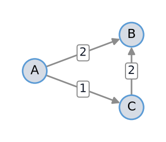

<Figure size 525x330 with 1 Axes> — Figure 1:The graph stored in `distance`, with the distance $c_{ij}$ along each arc $i \to j$ .

A pair of nodes without an arc simply has no key. In the mathematical models we then set $c_{ij} = \infty$ for a distance (the arc is never worth using) or $c_{ij} = 0$ for a capacity (nothing can flow through it).

References¶

Koole, G. (2019). An Introduction to Business Analytics. Chapter 7, “Combinatorial Optimization,” introduction.
Wolpert, D. H., & Macready, W. G. (1997). No free lunch theorems for optimization. IEEE Transactions on Evolutionary Computation, 1(1), 67-82.