
In the previous notebooks we solved the shortest path and maximum flow problems with fast exact algorithms, while for the traveling salesman problem we only found an exact algorithm that tries all tours, which takes far too long for large instances. Complexity theory is about the running times of algorithms, and it explains this difference. It also tells us what to expect in practice: whether a solver will find the optimal solution of a large instance, or whether a heuristic is the better choice. In the second part of this notebook we continue with the TSP example and solve it with a heuristic, the 2-opt heuristic.
Learning outcomes
On completion of this notebook, you will be able to:
explain the difference between polynomial and non-polynomial running-time growth, and why it matters in practice;
classify the problems of this course as belonging to P or being NP-complete, and explain the practical consequence of that classification;
explain why LO is efficiently solvable in practice although the simplex method is not polynomial;
distinguish metaheuristics from problem-specific heuristics;
apply the 2-opt heuristic by hand, and explain the difference between a local and a global optimum.
Running Time
The running time of an algorithm depends on the size of the instance, for example the number of nodes of a network. We count the number of basic operations the algorithm performs as a function of , and are only interested in how fast it grows. Some examples from this lecture:
Dijkstra’s algorithm repeats its loop times and looks at no more than nodes per repetition, so it takes about operations;
trying all tours of a TSP means checking tours, which takes about operations.
A precise count, for example operations with the number of operations to update one node, does not matter much: for large , the term determines the growth. We write that the running time is , “of the order ”. An algorithm is polynomial if its running time is for some fixed power , and non-polynomial otherwise, for example if it grows like or .
The difference is huge, as Table 1 shows.
Table 1:Values of polynomial and non-polynomial functions.
| 1 | 0 | 0 | 1 | 1 | 2 | 1 |
| 5 | 2.32 | 11.6 | 25 | 3125 | 32 | 120 |
| 10 | 3.32 | 33.2 | 100 | 105 | 1024 | |
| 20 | 4.32 | 86.4 | 400 | |||
| 50 | 5.64 | 282 | 2500 | |||
| 100 | 6.64 | 664 | 104 | 1010 | ||
| 1000 | 9.97 | 9966 | 106 | 1015 |
Suppose a computer performs a billion (109) operations per second. An algorithm with operations then solves an instance with in 10 seconds. An algorithm with operations takes about years for the same instance, thousands of times the age of the universe, and one with operations takes even longer: there are only about 1080 atoms in the universe. Faster computers do not help much. If computer power doubles every two years, as Moore’s law roughly says, a algorithm can handle one extra node every two years. A quantum computer could at best take the square root of these numbers for some problems, which still leaves .
P and NP-Complete
Researchers try to find polynomial algorithms for every problem. For some problems they succeeded, and proved that the algorithm always finds an optimal solution. For other problems, such as the TSP, hundreds of researchers have looked for a polynomial algorithm for decades without success. Based on the running time of the best known exact algorithm, there are, roughly speaking, two classes of problems.
P is the class of problems for which a polynomial exact algorithm is known. Optimal solutions can be found even for large instances. Examples are the transportation problem, the shortest path problem, the maximum flow problem, the product-mix problem and LO in general.
NP-complete problems are problems for which no polynomial exact algorithm is known. Large instances are solved with heuristics, or with solvers that may need a very long time to prove optimality. Examples are the knapsack problem, machine scheduling, set covering, the TSP and ILO in general.
The NP-complete problems are, in a precise sense, all equally hard: each of them can be translated into any other in polynomial time. So a polynomial algorithm for one NP-complete problem would give a polynomial algorithm for all of them.
For the modeling in this course, this means that adding integer variables to an LO model can change a problem that solves in a second into one that a solver cannot finish.
How to Win a Million Dollars
Whether NP-complete problems can be solved in polynomial time is an open question, known as “P versus NP”. It is one of the seven Millennium Prize Problems, for each of which the Clay Mathematics Institute offers US$1 million. To win, do one of the following:
find a polynomial exact algorithm for an NP-complete problem, or
prove that no polynomial exact algorithm exists for an NP-complete problem.
Most researchers believe that the second statement is true, but nobody has proved it. Of the seven Millennium Prize Problems, only the Poincaré conjecture has been officially solved so far, by Grigori Perelman in 2003. In September 2026, OpenAI claimed that its AI system had solved another one, the Navier-Stokes problem about the equations that describe how fluids flow (Nature, 2026). At the time of writing, mathematicians are still checking the proof.
Heuristics
For NP-complete problems such as the TSP, no polynomial exact algorithm is known. A heuristic does not aim for the optimum but for a near-optimal solution in a reasonable amount of time. There are two types:
Metaheuristics are not specific to one problem. Examples are local search, evolutionary algorithms, tabu search and simulated annealing. They still need some tailoring to the problem at hand, for example a definition of which solutions are “close” to each other.
Problem-specific heuristics use the structure of one problem. For common problems there is a lot of literature on them. The 2-opt heuristic for the TSP, below, is an example.
Before using a heuristic, ask whether you need the optimal solution at all, and how much worse than optimal a solution may be. A heuristic usually gives no guarantee about how far its solution is from the optimum, so it can be hard to tell whether a solution is good enough. Comparing heuristics on the same instances, or with a lower bound such as the value of an LO relaxation, helps.
The 2-Opt Heuristic
Local Search
The 2-opt heuristic is a local search method. Local search starts with some solution and repeatedly moves to a better solution close to the current one, until there is no better solution close by. “Close” is made precise by a neighborhood: for every solution , a set of solutions that can be reached from with one small change. Writing for the length of tour , local search is:
Start: an initial tour .
While contains a tour with :
.
The final tour has no better tour in its neighborhood: it is a local optimum. There is no guarantee that it is a global optimum, a best tour overall.
The 2-opt heuristic uses the TSP-specific neighborhood of all tours that can be reached from with one 2-opt swap:
remove two edges of the tour that do not share a node;
reconnect the two pieces into a tour, with the other two edges that do so.
There is only one other way to reconnect the pieces into one tour: if the tour goes and we remove the edges - and -, the new tour goes , where the part from to is now traveled in the opposite direction. The length changes by
so the swap is an improvement if this is negative. For the initial tour, a simple choice is to start at some node and repeatedly move to a random unvisited node.
Example
We continue with the example of
Traveling Salesman Problem, with the same distances and the
same function tour_length as there. A missing edge has distance .
import math

distance = {
    ("A", "B"): 2,
    ("A", "C"): 1,
    ("B", "C"): 2,
    ("B", "D"): 3,
    ("B", "E"): 2,
    ("C", "D"): 3,
    ("C", "E"): 6,
    ("D", "E"): 1,
    ("D", "F"): 5,
    ("E", "F"): 2,
}


def edge_length(i, j):
    """Distance between i and j, infinite if there is no edge."""
    return distance.get((i, j), distance.get((j, i), math.inf))


def tour_length(tour):
    """Total distance of a tour (list of nodes) back to its start."""
    return sum(edge_length(i, j) for i, j in zip(tour, tour[1:] + tour[:1]))
Source
import math

import matplotlib.pyplot as plt
from matplotlib.patches import Circle, FancyArrowPatch

# colors that read on the light and the dark site theme
NODE_FILL, NODE_EDGE = "#d6dce5", "#5b9bd5"
EDGE_COLOR, TEXT_COLOR = "#8c8c8c", "#111827"
NODE_RADIUS = 0.2


def draw_graph(
    positions,
    arcs,
    highlight=(),
    highlight_color="#d62728",
    directed=True,
    both_ways=(),
    label_at=None,
    node_notes=None,
    cut_x=None,
    figsize=(6, 3.2),
):
    """Draw a graph with a number (label) on every arc.

    positions: node -> (x, y)
    arcs: (i, j) -> label; both_ways: arcs drawn with an arrow at both ends
    highlight: arcs drawn thick in highlight_color
    label_at: (i, j) -> position of the label along the arc (default 0.5)
    node_notes: node -> (text, dx, dy) for a box next to the node
    cut_x: x-coordinate of a vertical line that marks a cut

    The background is transparent and every text sits on its own box, so
    the figure reads the same in the light and the dark site theme.
    """
    label_at = label_at or {}
    node_notes = node_notes or {}
    fig, ax = plt.subplots(figsize=figsize, dpi=150)
    fig.patch.set_alpha(0)
    ax.patch.set_alpha(0)
    for (i, j), label in arcs.items():
        (x1, y1), (x2, y2) = positions[i], positions[j]
        on = (i, j) in highlight or (not directed and (j, i) in highlight)
        color = highlight_color if on else EDGE_COLOR
        style = "-"
        if directed:
            style = "<|-|>" if (i, j) in both_ways else "-|>"
        # start and end the arc at the border of the node circles
        length = math.hypot(x2 - x1, y2 - y1)
        dx = (x2 - x1) / length * NODE_RADIUS
        dy = (y2 - y1) / length * NODE_RADIUS
        arrow = FancyArrowPatch(
            (x1 + dx, y1 + dy),
            (x2 - dx, y2 - dy),
            arrowstyle=style,
            mutation_scale=14,
            color=color,
            lw=3 if on else 1.5,
            shrinkA=0,
            shrinkB=0,
        )
        ax.add_patch(arrow)
        t = label_at.get((i, j), 0.5)
        ax.text(
            x1 + t * (x2 - x1),
            y1 + t * (y2 - y1),
            str(label),
            ha="center",
            va="center",
            fontsize=11,
            color=TEXT_COLOR,
            bbox={"boxstyle": "round,pad=0.2", "fc": "white", "ec": color},
        )
    for node, (x, y) in positions.items():
        circle = Circle(
            (x, y), NODE_RADIUS, fc=NODE_FILL, ec=NODE_EDGE, lw=1.5, zorder=3
        )
        ax.add_patch(circle)
        ax.text(x, y, node, ha="center", va="center", fontsize=12, zorder=4)
    for node, (text, dx, dy) in node_notes.items():
        x, y = positions[node]
        ax.text(
            x + dx,
            y + dy,
            text,
            ha="center",
            va="center",
            fontsize=11,
            color=highlight_color,
            fontweight="bold",
            bbox={
                "boxstyle": "round,pad=0.2",
                "fc": "white",
                "ec": highlight_color,
            },
        )
    xs = [x for x, _ in positions.values()]
    ys = [y for _, y in positions.values()]
    if cut_x is not None:
        ax.plot(
            [cut_x, cut_x],
            [min(ys) - 0.4, max(ys) + 0.4],
            color="#d62728",
            lw=3,
        )
    ax.set_xlim(min(xs) - 0.45, max(xs) + 0.45)
    ax.set_ylim(min(ys) - 0.45, max(ys) + 0.45)
    ax.set_aspect("equal")
    ax.axis("off")
    plt.show()


def tour_edges(tour):
    """The edges of a tour given as a list of nodes."""
    return {(tour[k], tour[(k + 1) % len(tour)]) for k in range(len(tour))}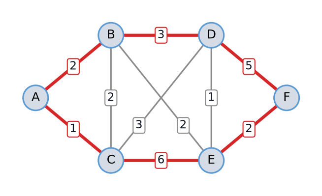
Figure 1:The TSP example network with the initial tour A → B → D → F → E → C → A of length 19 (red).
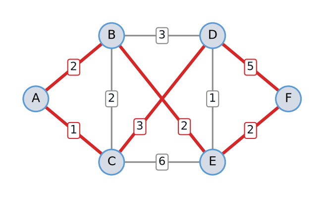
We start with the tour A → B → D → F → E → C → A of length 19 in Figure 1. Consider the swap that removes the edges B-D (length 3) and E-C (length 6). Reconnecting gives the edges B-E (length 2) and D-C (length 3), and the length changes by . The new tour A → B → E → F → D → C → A in Figure 2 has length 15: the part D → F → E is now traveled as E → F → D. No 2-opt swap improves this tour, so it is a local optimum. Here it is also a global optimum: in Traveling Salesman Problem, pulp and brute force found the same length.
2-Opt in Python
The function better_neighbor goes through all 2-opt swaps of a tour and returns
the first tour in its neighborhood that is shorter, or None if there is none. A
swap that removes the edges after positions i and j reverses the part of the
tour in between. The loop at the bottom is the local search algorithm above.
def better_neighbor(tour):
    """First tour in the 2-opt neighborhood of tour that is shorter."""
    n = len(tour)
    for i in range(n - 1):
        for j in range(i + 2, n):
            if i == 0 and j == n - 1:
                continue  # these two edges share the start node
            neighbor = (
                tour[: i + 1] + tour[i + 1 : j + 1][::-1] + tour[j + 1 :]
            )
            if tour_length(neighbor) < tour_length(tour):
                return neighbor
    return None


tour = ["A", "B", "D", "F", "E", "C"]
print("initial tour:", "".join(tour), "length", tour_length(tour))
neighbor = better_neighbor(tour)
while neighbor is not None:
    tour = neighbor
    print("better tour: ", "".join(tour), "length", tour_length(tour))
    neighbor = better_neighbor(tour)
print("local optimum:", "".join(tour))
initial tour: ABDFEC length 19
better tour: ABEFDC length 15
local optimum: ABEFDC
Local and Global Optima
How good the local optimum is depends on the initial tour and on the neighborhood. Starting from another initial tour can end in another local optimum, so a common approach is to run the heuristic from several initial tours and keep the best result. A larger neighborhood gives better local optima, but takes longer to search. The 3-opt heuristic removes three edges and tries all ways of reconnecting the pieces, and is known to give better tours than 2-opt. In general, the -opt neighborhood removes edges and contains in the order of tours.
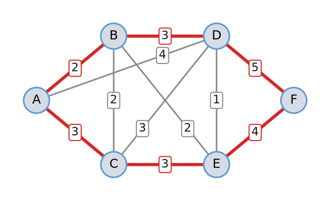
Figure 3:Undirected graph of Exercise 1, with distances along the edges.
References
Koole, G. (2019). An Introduction to Business Analytics. Chapter 7, “Combinatorial Optimization” (complexity, heuristics).