
The second classical problem of this lecture is the maximum flow problem: how much can be sent through a network from one node to another when every arc has a capacity? As for the shortest path problem, and next for the traveling salesman problem, we define the problem and give an example, solve the example with an LO approach, and then solve it with a dedicated algorithm: the Ford-Fulkerson algorithm. As usual, the dedicated algorithm is often the way to go in practice. A cut then gives a simple test of whether a flow is maximal.
Learning outcomes
On completion of this notebook, you will be able to:
formulate the maximum flow problem as an LO model and solve it with pulp;
find augmenting paths, including paths that use an arc backwards, and apply the Ford-Fulkerson algorithm by hand;
compute the value of a cut and use a cut to show that a flow is maximal.
The Maximum Flow Problem
How much traffic can flow per hour from one part of a city to another, and which roads are the bottlenecks? Questions like this one are maximum flow problems. Other examples are whether the supply in a network can meet the demand given the capacities of the connections, and planning in which a limited resource has to be divided, such as crews in airline scheduling.
Given are a directed graph with a source node , a destination node , and a flow capacity on every arc : no more than can flow from to . The goal is to find the maximum flow from to that respects
the capacities: the flow on an arc is at most its capacity;
flow conservation: what flows into a node also flows out of it, except at and .
This is similar to the transshipment problem with one warehouse and one customer, where the goal is now to deliver as much as possible and the arcs have capacities instead of costs.
As an example, we look for the maximum flow from to in Figure 1. The capacity means that at most 4 can flow from D to F. A pair of nodes without an arc, such as A and D, has capacity .
Source
import math

import matplotlib.pyplot as plt
from matplotlib.patches import Circle, FancyArrowPatch

# colors that read on the light and the dark site theme
NODE_FILL, NODE_EDGE = "#d6dce5", "#5b9bd5"
EDGE_COLOR, TEXT_COLOR = "#8c8c8c", "#111827"
NODE_RADIUS = 0.2


def draw_graph(
    positions,
    arcs,
    highlight=(),
    highlight_color="#d62728",
    directed=True,
    both_ways=(),
    label_at=None,
    node_notes=None,
    cut_x=None,
    figsize=(6, 3.2),
):
    """Draw a graph with a number (label) on every arc.

    positions: node -> (x, y)
    arcs: (i, j) -> label; both_ways: arcs drawn with an arrow at both ends
    highlight: arcs drawn thick in highlight_color
    label_at: (i, j) -> position of the label along the arc (default 0.5)
    node_notes: node -> (text, dx, dy) for a box next to the node
    cut_x: x-coordinate of a vertical line that marks a cut

    The background is transparent and every text sits on its own box, so
    the figure reads the same in the light and the dark site theme.
    """
    label_at = label_at or {}
    node_notes = node_notes or {}
    fig, ax = plt.subplots(figsize=figsize, dpi=150)
    fig.patch.set_alpha(0)
    ax.patch.set_alpha(0)
    for (i, j), label in arcs.items():
        (x1, y1), (x2, y2) = positions[i], positions[j]
        on = (i, j) in highlight or (not directed and (j, i) in highlight)
        color = highlight_color if on else EDGE_COLOR
        style = "-"
        if directed:
            style = "<|-|>" if (i, j) in both_ways else "-|>"
        # start and end the arc at the border of the node circles
        length = math.hypot(x2 - x1, y2 - y1)
        dx = (x2 - x1) / length * NODE_RADIUS
        dy = (y2 - y1) / length * NODE_RADIUS
        arrow = FancyArrowPatch(
            (x1 + dx, y1 + dy),
            (x2 - dx, y2 - dy),
            arrowstyle=style,
            mutation_scale=14,
            color=color,
            lw=3 if on else 1.5,
            shrinkA=0,
            shrinkB=0,
        )
        ax.add_patch(arrow)
        t = label_at.get((i, j), 0.5)
        ax.text(
            x1 + t * (x2 - x1),
            y1 + t * (y2 - y1),
            str(label),
            ha="center",
            va="center",
            fontsize=11,
            color=TEXT_COLOR,
            bbox={"boxstyle": "round,pad=0.2", "fc": "white", "ec": color},
        )
    for node, (x, y) in positions.items():
        circle = Circle(
            (x, y), NODE_RADIUS, fc=NODE_FILL, ec=NODE_EDGE, lw=1.5, zorder=3
        )
        ax.add_patch(circle)
        ax.text(x, y, node, ha="center", va="center", fontsize=12, zorder=4)
    for node, (text, dx, dy) in node_notes.items():
        x, y = positions[node]
        ax.text(
            x + dx,
            y + dy,
            text,
            ha="center",
            va="center",
            fontsize=11,
            color=highlight_color,
            fontweight="bold",
            bbox={
                "boxstyle": "round,pad=0.2",
                "fc": "white",
                "ec": highlight_color,
            },
        )
    xs = [x for x, _ in positions.values()]
    ys = [y for _, y in positions.values()]
    if cut_x is not None:
        ax.plot(
            [cut_x, cut_x],
            [min(ys) - 0.4, max(ys) + 0.4],
            color="#d62728",
            lw=3,
        )
    ax.set_xlim(min(xs) - 0.45, max(xs) + 0.45)
    ax.set_ylim(min(ys) - 0.45, max(ys) + 0.45)
    ax.set_aspect("equal")
    ax.axis("off")
    plt.show()


def flow_labels(capacity, flow):
    """Arc labels flow/capacity."""
    return {arc: f"{flow[arc]}/{cap}" for arc, cap in capacity.items()}


def augment_and_draw(positions, capacity, flow, path):
    """Increase the flow along path (a list of nodes) and draw the result.

    A step i -> j uses the arc i -> j forward if it exists, and otherwise
    the arc j -> i backwards. The augmenting path is drawn in green.
    """
    steps = []
    for i, j in zip(path, path[1:]):
        if (i, j) in capacity:
            steps.append(((i, j), capacity[i, j] - flow[i, j], +1))
        else:
            steps.append(((j, i), flow[j, i], -1))
    delta = min(room for _, room, _ in steps)
    for arc, _, direction in steps:
        flow[arc] += direction * delta
    draw_graph(
        positions,
        flow_labels(capacity, flow),
        highlight={arc for arc, _, _ in steps},
        highlight_color="#2ca02c",
    )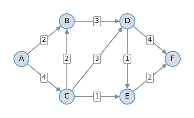
Figure 1:Example network with flow capacities along the arcs.
LO Approach
Model
Decision Variables
= the flow from to , for all .
Objective
Maximize the flow out of the source, . By flow conservation, everything that leaves the source arrives at the destination, so maximizing gives the same answer. If there are arcs into the source, maximize the net outflow instead: otherwise flow could go round in a cycle back to the source and count twice.
Constraints
The flow on an arc is at most its capacity, every node other than and has flow in equal to flow out, and flows are non-negative.
Complete LO Model
Model for the Example
For Figure 1, with source A and destination F, we only need variables for the 9 arcs: a pair without an arc has capacity 0, so its flow is 0. No arc enters A, so the objective is the flow out of A.
Solving the Example in pulp
As for the shortest path problem, we only create variables for arcs that exist. New
is the upBound argument of pulp.LpVariable: it gives a variable an upper bound,
here the capacity, so the capacity constraints need no separate lines.
import pulp

capacity = {
    ("A", "B"): 2,
    ("A", "C"): 4,
    ("B", "D"): 3,
    ("C", "B"): 2,
    ("C", "D"): 3,
    ("C", "E"): 1,
    ("D", "E"): 1,
    ("D", "F"): 4,
    ("E", "F"): 2,
}
nodes = ["A", "B", "C", "D", "E", "F"]
source, destination = "A", "F"

max_flow = pulp.LpProblem(name="max_flow", sense=pulp.LpMaximize)
send = {
    (i, j): pulp.LpVariable(name=f"x_{i}_{j}", lowBound=0, upBound=cap)
    for (i, j), cap in capacity.items()
}

max_flow += pulp.lpSum(send[i, j] for (i, j) in capacity if i == source)
for k in nodes:
    if k in (source, destination):
        continue
    inflow = pulp.lpSum(send[i, j] for (i, j) in capacity if j == k)
    outflow = pulp.lpSum(send[i, j] for (i, j) in capacity if i == k)
    max_flow += inflow == outflow, f"conservation_{k}"

max_flow.solve(pulp.PULP_CBC_CMD(msg=False))
print("status:", pulp.LpStatus[max_flow.status])
print("flows:", {a: v.value() for a, v in send.items() if v.value() > 0})
print("maximum flow:", max_flow.objective.value())
status: Optimal
flows: {('A', 'B'): 2.0, ('A', 'C'): 4.0, ('B', 'D'): 3.0, ('C', 'B'): 1.0, ('C', 'D'): 2.0, ('C', 'E'): 1.0, ('D', 'E'): 1.0, ('D', 'F'): 4.0, ('E', 'F'): 2.0}
maximum flow: 6.0
The maximum flow is 6. How can we see that without a solver, and how can we be sure that no larger flow exists? That is what the Ford-Fulkerson algorithm and cuts are for.
The Ford-Fulkerson Algorithm
Augmenting Paths
Suppose we have a flow that respects the capacities and flow conservation, for example on all arcs. An augmenting path is a path from to that consists only of
forward arcs whose capacity is not reached, , and
reversed arcs: arcs with positive flow, , used backwards, from to .
The key idea is that the flow from to can be increased along an augmenting path: increase the flow on every forward arc and decrease the flow on every reversed arc, by the same amount . Every node on the path then keeps flow in equal to flow out, and receives more. Decreasing the flow on a reversed arc means that flow which first went from to is redirected: node sends it along the rest of the augmenting path instead, and node receives the new flow from the path in its place.
How large can be? A forward arc has room for more, and the flow on a reversed arc can decrease by at most . So the largest value is
determined by the bottleneck of the path. These remaining amounts, forward and backward, are the available remaining capacities considering the current flow: together they form the so-called residual graph, and an augmenting path is a path from to in it.
The Algorithm
Start: for all arcs.
While there is an augmenting path from to :
Find an augmenting path and its maximum increase in flow .
Increase the flow along the path: on its forward arcs and on its reversed arcs. This updates the available capacities.
When no augmenting path can be found, the flow is maximal. Why that is the case follows from cuts below.
Example
We apply the algorithm to Figure 1. In the figures below, the label of an arc gives its flow and capacity, and the augmenting path is green.
Iteration 1. All flows are 0, so any path from A to F is augmenting. We take A → B → D → E → F. Its bottleneck is , the capacity of D → E. After increasing the flow, the total flow is 1 (Figure 2).
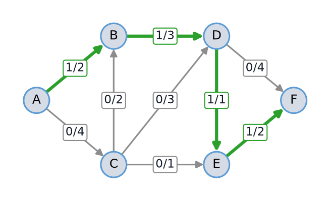
Figure 2:Iteration 1 of Ford-Fulkerson: flow 1 along A → B → D → E → F.
Iteration 2. A → C → B → D → F is augmenting: A → C has room 4, C → B room 2, B → D room and D → F room 4. So , and the total flow becomes 3 (Figure 3).
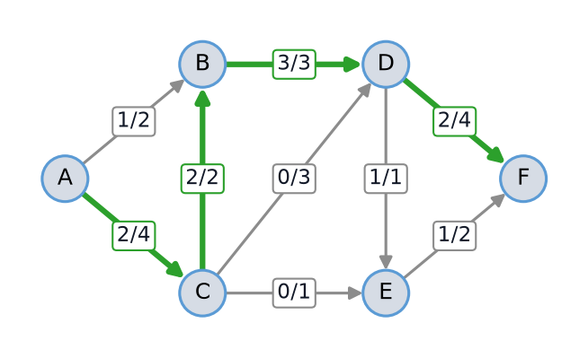
Figure 3:Iteration 2 of Ford-Fulkerson: flow 2 along A → C → B → D → F.
Iteration 3. A → C → D → F has rooms , 3 and , so , and the total flow becomes 5 (Figure 4).
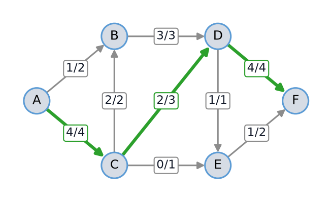
Figure 4:Iteration 3 of Ford-Fulkerson: flow 2 along A → C → D → F.
Iteration 4. Now A → C, B → D and D → F are full, so a path that only uses forward arcs no longer exists. An augmenting path can also send flow backwards, though: A → B → C → E → F uses the arc C → B backwards. A → B has room , the flow 2 on C → B can decrease by 2, C → E has room 1 and E → F room , so . The flow on C → B decreases from 2 to 1: one unit that went from C to B now goes from C to E, and B receives a unit from A in its place. The total flow becomes 6 (Figure 5).
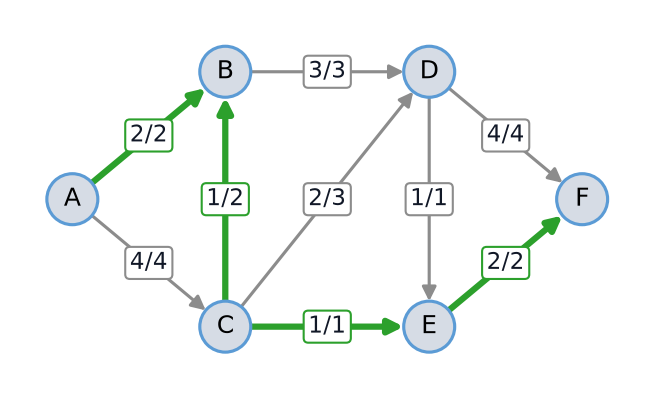
Figure 5:Iteration 4 of Ford-Fulkerson: flow 1 along A → B → C → E → F, where the arc C → B is used backwards, so its flow decreases from 2 to 1.
Iteration 5. Both arcs out of A are full, and A has no arcs into it that carry flow, so we cannot even leave A: there is no augmenting path. The algorithm stops with a flow of 6, the same value as pulp found.
Other choices of augmenting paths are possible and lead to the same maximum flow, possibly with different flows on the arcs.
Cuts: Checking That a Flow Is Maximal
A cut splits the nodes into a set that contains the source and the rest that contains the destination. The value of the cut is the total capacity of the arcs from a node in to a node outside :
Cutting these arcs disconnects every path from to . Every unit of flow from to has to cross from to the rest over one of them, so
Arcs that point into do not count in . Flow over such an arc goes back into , so it has to cross from to the rest once more: it can only lower the net amount that leaves , never raise it. For example, in Figure 1 the cut consists of A → C and B → D and has value . The arc C → B also connects with the rest, but it points into , so its capacity does not count. Every cut gives an upper bound on the flow, and some bounds are better than others: the cut has value , a weaker bound than 7.
The inequality above already gives an optimality test: if we find a flow and a cut with the same value, no flow can be larger than this flow, so it is maximal (and no cut can be smaller, so the cut is minimal). The max-flow min-cut theorem adds that such a cut always exists: the maximum flow from to equals the minimum value of an - cut. So for a maximum flow, the optimality test always works: there is always a cut with the same value.
When the Ford-Fulkerson algorithm stops, such a cut is easy to find: let be the set of nodes that can still be reached from along forward arcs with room and reversed arcs with flow. All arcs from to the rest are full, and all arcs into are empty, so the flow equals . That is also why the algorithm finds a maximum flow. In the example, no node can be reached from A, so , with value (Figure 6). This equals the flow of 6, so the flow is maximal.
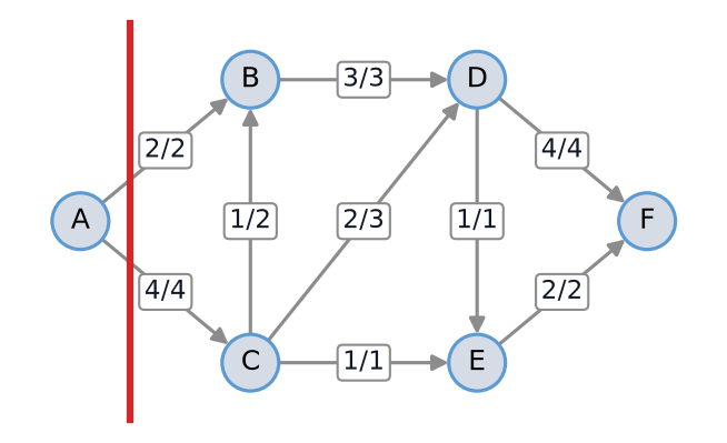
Figure 6:The final flow with the cut (red line), with value , equal to the flow.
Ford-Fulkerson in Python
The function augmenting_path searches for an augmenting path from the source,
node by node: from a node it continues over every arc with room left
(forward) and every arc with positive flow (reversed). It returns the
path as a list of steps (arc, direction), with direction +1 for a forward and
-1 for a reversed arc, and also the set of nodes it could reach, which is the
minimum cut once no path exists. The function ford_fulkerson follows the
algorithm above. As for Dijkstra’s algorithm, you do not have to be able to write
this code yourself, but you should be able to follow what each line does.
def augmenting_path(capacity, flow, source, destination):
    """Search an augmenting path; return it and the reachable nodes."""
    path_to = {source: []}
    to_explore = [source]
    while to_explore:
        i = to_explore.pop(0)
        for (a, b), cap in capacity.items():
            if a == i and b not in path_to and flow[a, b] < cap:
                path_to[b] = path_to[i] + [((a, b), +1)]
                to_explore.append(b)
            elif b == i and a not in path_to and flow[a, b] > 0:
                path_to[a] = path_to[i] + [((a, b), -1)]
                to_explore.append(a)
    return path_to.get(destination), set(path_to)


def ford_fulkerson(capacity, source, destination):
    """Maximum flow with the Ford-Fulkerson algorithm."""
    flow = {arc: 0 for arc in capacity}
    path, reached = augmenting_path(capacity, flow, source, destination)
    while path is not None:
        room = [
            capacity[arc] - flow[arc] if direction == 1 else flow[arc]
            for arc, direction in path
        ]
        delta = min(room)
        for arc, direction in path:
            flow[arc] += direction * delta
        visits = [source] + [a if dr == -1 else b for (a, b), dr in path]
        print(f"augmenting path {' -> '.join(visits)}, delta = {delta}")
        path, reached = augmenting_path(capacity, flow, source, destination)
    return flow, reached


ff_flow, cut_side = ford_fulkerson(capacity, source, destination)
flow_value = sum(ff_flow[i, j] for (i, j) in capacity if i == source)
cut_value = sum(
    cap
    for (i, j), cap in capacity.items()
    if i in cut_side and j not in cut_side
)
print("maximum flow:", flow_value)
print("minimum cut S:", sorted(cut_side), "with value", cut_value)
augmenting path A -> B -> D -> F, delta = 2
augmenting path A -> C -> D -> F, delta = 2
augmenting path A -> C -> E -> F, delta = 1
augmenting path A -> C -> D -> E -> F, delta = 1
maximum flow: 6
minimum cut S: ['A'] with value 6
The function finds different augmenting paths than we chose by hand, with the same maximum flow of 6.
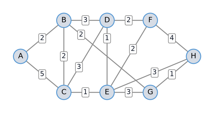
Figure 7:Undirected graph of Exercise 2, with capacities along the edges.
Running Time
The running time of the Ford-Fulkerson algorithm is , where is the value of the maximum flow and the number of arcs (the notation is explained in Complexity and Heuristics). The algorithm repeats its loop as long as there is an augmenting path, and finding one looks at every arc a few times. With integer capacities, every iteration increases the flow by at least 1, so in the worst case there are iterations. More refined implementations, which choose the augmenting paths more carefully, have a polynomial running time.
References
Koole, G. (2019). An Introduction to Business Analytics. Chapter 7, “Combinatorial Optimization” (maximum flow).