
This notebook is the first of the three problem notebooks of this lecture, introduced in Algorithms and Their Characteristics. We define the shortest path problem, solve an example with an LO model in pulp, and then solve it with Dijkstra’s algorithm, the dedicated algorithm for this problem.
Learning outcomes
On completion of this notebook, you will be able to:
formulate the shortest path problem as an LO model and solve it with pulp;
explain what means at every step of Dijkstra’s algorithm;
apply Dijkstra’s algorithm by hand in a table and find a shortest path by backtracking;
explain why Dijkstra’s algorithm needs non-negative distances and why its running time grows like .
The Shortest Path Problem
Every time you ask navigation software for a route, it solves a shortest path problem: find the shortest (or fastest) route from where you are to where you want to go. The same problem appears in many less visible places, for example in routing data packets through the internet, and as a building block of other problems: the traveling salesman problem needs the shortest distance between every pair of cities.
In the notation of Graphs: Notation for This Lecture, the problem is: given a directed graph with distances on the arcs, find a shortest path from a source node to a destination node . An undirected edge, which can be used in both directions, counts as two arcs.
As an example, we look for a shortest path from to in the graph of Figure 1. For example, the distance from D to F is , and the edge between B and C can be used in both directions: .
Source
import math

import matplotlib.pyplot as plt
from matplotlib.patches import Circle, FancyArrowPatch

# colors that read on the light and the dark site theme
NODE_FILL, NODE_EDGE = "#d6dce5", "#5b9bd5"
EDGE_COLOR, TEXT_COLOR = "#8c8c8c", "#111827"
NODE_RADIUS = 0.2


def draw_graph(
    positions,
    arcs,
    highlight=(),
    highlight_color="#d62728",
    directed=True,
    both_ways=(),
    label_at=None,
    node_notes=None,
    cut_x=None,
    figsize=(6, 3.2),
):
    """Draw a graph with a number (label) on every arc.

    positions: node -> (x, y)
    arcs: (i, j) -> label; both_ways: arcs drawn with an arrow at both ends
    highlight: arcs drawn thick in highlight_color
    label_at: (i, j) -> position of the label along the arc (default 0.5)
    node_notes: node -> (text, dx, dy) for a box next to the node
    cut_x: x-coordinate of a vertical line that marks a cut

    The background is transparent and every text sits on its own box, so
    the figure reads the same in the light and the dark site theme.
    """
    label_at = label_at or {}
    node_notes = node_notes or {}
    fig, ax = plt.subplots(figsize=figsize, dpi=150)
    fig.patch.set_alpha(0)
    ax.patch.set_alpha(0)
    for (i, j), label in arcs.items():
        (x1, y1), (x2, y2) = positions[i], positions[j]
        on = (i, j) in highlight or (not directed and (j, i) in highlight)
        color = highlight_color if on else EDGE_COLOR
        style = "-"
        if directed:
            style = "<|-|>" if (i, j) in both_ways else "-|>"
        # start and end the arc at the border of the node circles
        length = math.hypot(x2 - x1, y2 - y1)
        dx = (x2 - x1) / length * NODE_RADIUS
        dy = (y2 - y1) / length * NODE_RADIUS
        arrow = FancyArrowPatch(
            (x1 + dx, y1 + dy),
            (x2 - dx, y2 - dy),
            arrowstyle=style,
            mutation_scale=14,
            color=color,
            lw=3 if on else 1.5,
            shrinkA=0,
            shrinkB=0,
        )
        ax.add_patch(arrow)
        t = label_at.get((i, j), 0.5)
        ax.text(
            x1 + t * (x2 - x1),
            y1 + t * (y2 - y1),
            str(label),
            ha="center",
            va="center",
            fontsize=11,
            color=TEXT_COLOR,
            bbox={"boxstyle": "round,pad=0.2", "fc": "white", "ec": color},
        )
    for node, (x, y) in positions.items():
        circle = Circle(
            (x, y), NODE_RADIUS, fc=NODE_FILL, ec=NODE_EDGE, lw=1.5, zorder=3
        )
        ax.add_patch(circle)
        ax.text(x, y, node, ha="center", va="center", fontsize=12, zorder=4)
    for node, (text, dx, dy) in node_notes.items():
        x, y = positions[node]
        ax.text(
            x + dx,
            y + dy,
            text,
            ha="center",
            va="center",
            fontsize=11,
            color=highlight_color,
            fontweight="bold",
            bbox={
                "boxstyle": "round,pad=0.2",
                "fc": "white",
                "ec": highlight_color,
            },
        )
    xs = [x for x, _ in positions.values()]
    ys = [y for _, y in positions.values()]
    if cut_x is not None:
        ax.plot(
            [cut_x, cut_x],
            [min(ys) - 0.4, max(ys) + 0.4],
            color="#d62728",
            lw=3,
        )
    ax.set_xlim(min(xs) - 0.45, max(xs) + 0.45)
    ax.set_ylim(min(ys) - 0.45, max(ys) + 0.45)
    ax.set_aspect("equal")
    ax.axis("off")
    plt.show()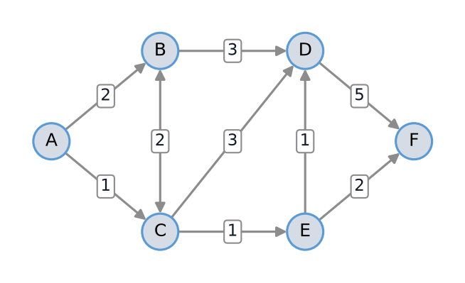
Figure 1:Example network with distances along the arcs. The edge between B and C can be used in both directions.
LO Approach
Model
The shortest path problem is a special case of the transshipment problem: ship one unit from the source (supply 1) to the destination (demand 1) as cheaply as possible, where the cost of using an arc is its distance. The unit follows a path, and the cost is the length of that path.
Decision Variables
if the arc is on the path, and 0 otherwise.
Objective
Minimize the length of the path, , with if there is no arc .
Constraints
One unit more leaves the source than enters it, one unit more enters the destination than leaves it, and every other node passes on what it receives (flow conservation). The constraint is needed: without it, a negative amount could flow backwards over an arc.
We do not require . As for the transportation problem, the corner points of the feasible region are already integer, so the simplex method returns a 0/1 solution. If a solver does return a fractional solution, the unit is split over several paths, and each of these paths is then a shortest path.
Complete LO Model
One of these constraints is redundant. Every arc leaves one node and enters another, so the net outflows (outflow minus inflow) of all nodes add up to 0. If the source has net outflow 1 and every other node except the destination has net outflow 0, the destination must have net outflow -1: it receives one unit. The destination constraint therefore follows from the others. We keep it because it makes the model easier to read, and it does not change the optimal solution.
Model for the Example
For Figure 1, with source A and destination F, there is a variable for each of the 10 arcs; pairs of nodes without an arc have , so their variables are 0 in any optimal solution and can be left out. No arc enters A or leaves F, which simplifies their constraints:
Solving the Example in pulp
The model is built as the transshipment model in
Transportation and Transshipment: the keys of the
dictionary distance are the arcs, and a variable is only created for an arc that
exists. The constraint of a node depends on whether it is the source, the
destination, or another node.
import pulp

distance = {
    ("A", "B"): 2,
    ("A", "C"): 1,
    ("B", "C"): 2,
    ("C", "B"): 2,
    ("B", "D"): 3,
    ("C", "D"): 3,
    ("C", "E"): 1,
    ("E", "D"): 1,
    ("D", "F"): 5,
    ("E", "F"): 2,
}
nodes = ["A", "B", "C", "D", "E", "F"]
source, destination = "A", "F"

shortest_path = pulp.LpProblem(name="shortest_path", sense=pulp.LpMinimize)
use = {
    (i, j): pulp.LpVariable(name=f"x_{i}_{j}", lowBound=0)
    for (i, j) in distance
}

shortest_path += pulp.lpSum(distance[a] * use[a] for a in distance)
for k in nodes:
    inflow = pulp.lpSum(use[i, j] for (i, j) in distance if j == k)
    outflow = pulp.lpSum(use[i, j] for (i, j) in distance if i == k)
    if k == source:
        shortest_path += outflow - inflow == 1, f"source_{k}"
    elif k == destination:
        shortest_path += inflow - outflow == 1, f"destination_{k}"
    else:
        shortest_path += inflow == outflow, f"conservation_{k}"

shortest_path.solve(pulp.PULP_CBC_CMD(msg=False))
print("status:", pulp.LpStatus[shortest_path.status])
print("arcs used:", [a for a in distance if use[a].value() > 0.5])
print("length:", shortest_path.objective.value())
status: Optimal
arcs used: [('A', 'C'), ('C', 'E'), ('E', 'F')]
length: 4.0
The shortest path is A → C → E → F, with length . The model has a variable for every arc and a constraint for every node. For a network with nodes where (almost) every pair of nodes is connected, that is about variables. Dijkstra’s algorithm finds the answer much faster.
Dijkstra’s Algorithm
Edsger Dijkstra (1930-2002) was a Dutch computer scientist. He designed his algorithm while working at the Mathematisch Centrum in Amsterdam, now the CWI (Centrum Wiskunde & Informatica), the Dutch national research institute for mathematics and computer science at Amsterdam Science Park. He published it in a three-page paper (Dijkstra, 1959). The algorithm finds the shortest paths from the source to all nodes at once, and it requires that all distances are non-negative, .
The idea is to grow a set of visited nodes, one node at a time. In every step we visit the nearest unvisited node, nearest in the sense of the shortest path that only passes through visited nodes. Dijkstra proved that once a node is visited, we know a shortest path from the source to that node.
What the Algorithm Keeps Track Of
To make every intermediate step precise, we define for a set of visited nodes and every node :
“Intermediate” means the nodes between the source and ; the source and themselves need not be in . If there is no such path, . For example, in Figure 1 with only the direct arcs from A count: , and for the other nodes. With , the path A → C → E is allowed too, so .
As grows, more paths are allowed and can only decrease. When contains all nodes, every path is allowed, so our aim is .
The Algorithm
Write for the set without the node .
Start: , and for all other nodes .
While does not contain all nodes:
Find the node with the smallest ; call it .
Visit : add it to . This makes the current node.
Update, for all :
When the first term is the smaller one, save as the previous node of .
The update considers the two possibilities for a shortest path to now that may be used as an intermediate node: the path goes via (first reach , then take the arc ), or it does not use and the old value stays. Only arcs out of can give an improvement, so in practice we only check the unvisited neighbors of the current node, with for the others.
The previous nodes give the shortest paths themselves: follow them backwards from the destination to the source.
As written, the algorithm finds the shortest paths from the source to all nodes. If you only need a shortest path to the destination, you can stop as soon as the destination is visited: its value is then final (see Why It Works).
Example
We apply the algorithm to Figure 1. Table 1 shows for every node throughout the algorithm, with the previous node in brackets. Each row shows the values after updating, for the nodes that are not yet visited, with the set of visited nodes in that row. The smallest of these values is underlined: its node becomes the current node in the next step.
Table 1:Distances throughout Dijkstra’s algorithm, from A, for the network in Figure 1.
| step | |||||||
|---|---|---|---|---|---|---|---|
| start | 0 | ∞ | ∞ | ∞ | ∞ | ∞ | |
| 1 | 2 (A) | 1 (A) | ∞ | ∞ | ∞ | ||
| 2 | 2 (A) | 4 (C) | 2 (C) | ∞ | |||
| 3 | 4 (C) | 2 © | ∞ | ||||
| 4 | 3 (E) | 4 (E) | |||||
| 5 | 4 (E) | ||||||
| 6 |
Step by step:
Start. Only the source has a finite value, so A becomes current.
Step 1. Visit A, so . Update the neighbors of A: and , both with previous node A. The smallest value among the unvisited nodes is 1, so C becomes current.
Step 2. Visit C. Via C, B could be reached in , which is worse than 2, so B keeps its value. D gets and E gets , both via C. B and E are tied at 2; we pick B (any choice works, see Exercise 1).
Step 3. Visit B. Via B, D could be reached in , so nothing changes, and E becomes current.
Step 4. Visit E. Via E, D is reached in , so with previous node E. F gets .
Step 5. Visit D. Via D, F could be reached in , so F keeps 4 and becomes current.
Step 6. Visit F. All nodes are in , so we stop.
Once a node is chosen as current node, its value does not change anymore, and it is the length of a shortest path from A to that node (see Why It Works). So the shortest distance of a node is the underlined value in its column. For example, D is chosen in the row of step 4, where and , so the shortest path from A to D has length 3. In the same way, the underlined in the row of step 5 is the length of a shortest path from A to F. Backtracking through the previous nodes gives the paths: the previous node of F is E, that of E is C, and that of C is A, so the shortest path from A to F is A → C → E → F, the same as pulp found. Together, the previous nodes form a tree of shortest paths from A to all nodes, shown in Figure 2.
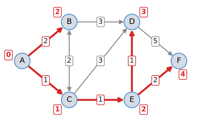
Figure 2:Result of Dijkstra’s algorithm from A: next to each node its shortest distance from A, and in red the arcs from each node’s previous node, which form the tree of shortest paths.
Why It Works
Suppose has the smallest value among the unvisited nodes. Any path from the source to that is not counted in leaves the visited nodes at some point: it reaches a first node outside , and then continues to . The part up to is at least long, and because all distances are non-negative, the rest of the path cannot make it shorter. So no path to is shorter than , and visiting fixes its shortest distance for good.
This argument fails with negative distances: a path could first go to a far-away node and then come back over an arc with a large negative distance. That is why Dijkstra’s algorithm requires . The argument also shows why we may stop as soon as the destination is visited: we then already know its shortest distance.
Dijkstra’s Algorithm in Python
The function below follows the algorithm line by line. You do not have to be able
to write it yourself, but read it next to The Algorithm and
check that you can follow each step. The dictionary d holds and the
list W the visited nodes. To show the steps, the function also builds the table
of Table 1.
import math

import pandas as pd


def dijkstra(nodes, distance, source):
    """Shortest distances from source with Dijkstra's algorithm.

    Returns d (node -> shortest distance), previous (node -> previous node
    on a shortest path) and the table of all steps.
    """
    d = {x: math.inf for x in nodes}
    d[source] = 0
    previous = {}
    W = []
    rows = []
    while len(W) < len(nodes):
        # 1. find the unvisited node with the smallest d_W(x)
        current = min((x for x in nodes if x not in W), key=lambda x: d[x])
        rows.append(table_row(nodes, d, previous, W, current))
        # 2. visit it
        W.append(current)
        # 3. update the unvisited nodes via the current node
        for x in nodes:
            if x not in W and (current, x) in distance:
                via_current = d[current] + distance[current, x]
                if via_current < d[x]:
                    d[x] = via_current
                    previous[x] = current
    rows.append(table_row(nodes, d, previous, W, ""))
    table = pd.DataFrame(rows)
    table.index = ["start"] + [f"step {k}" for k in range(1, len(rows))]
    return d, previous, table


def table_row(nodes, d, previous, W, current):
    """One row of the table: d_W(x) (previous node) for unvisited x."""
    row = {}
    for x in nodes:
        if x in W:
            row[x] = ""
        elif x in previous:
            row[x] = f"{d[x]} ({previous[x]})"
        else:
            row[x] = "∞" if d[x] == math.inf else str(d[x])
    row["current"] = current
    row["W"] = "{" + ", ".join(W) + "}"
    return row


d, previous, table = dijkstra(nodes, distance, source)
tableBacktracking through previous gives the shortest path:
path = [destination]
while path[0] != source:
    path.insert(0, previous[path[0]])
print("shortest path:", " -> ".join(path), "with length", d[destination])
shortest path: A -> C -> E -> F with length 4
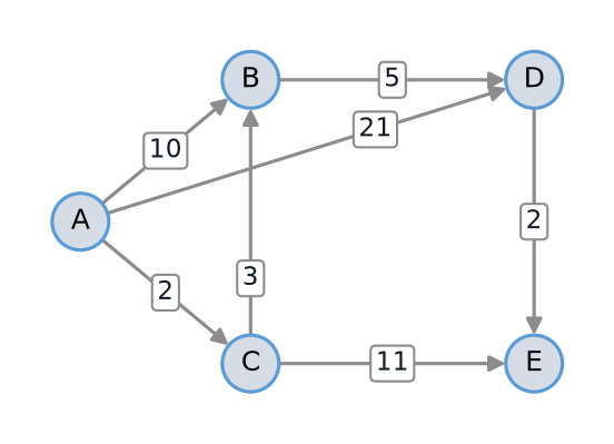
Figure 3:Directed graph of Exercise 3, with distances along the arcs.
Running Time
How much work does Dijkstra’s algorithm take for a network with nodes? Every repetition of the while loop visits one new node, so there are repetitions. In each repetition, finding the unvisited node with the smallest value and updating the unvisited nodes each look at no more than nodes. In total that is about operations. For a network with 1000 nodes, this is in the order of a million operations, a fraction of a second on a computer. In Complexity and Heuristics we compare this with problems for which no such fast algorithm is known.
References
Koole, G. (2019). An Introduction to Business Analytics. Chapter 7, “Combinatorial Optimization” (shortest path).
Dijkstra, E. W. (1959). A note on two problems in connexion with graphs. Numerische Mathematik, 1, 269-271.