
The third classical problem of this lecture is the traveling salesman problem (TSP): find the shortest tour along a number of cities. As for the shortest path and maximum flow problems, we define the problem and give an example, solve the example with an ILO approach, and then look for a dedicated algorithm. This time the story ends differently. The ILO model needs a huge number of constraints, and the only exact algorithm we find tries all tours, which takes far too long for large instances. No exact algorithm with a polynomial running time is known for the TSP. The next notebook, Complexity and Heuristics, explains what that means and why, and continues with this example using a heuristic.
Learning outcomes
On completion of this notebook, you will be able to:
formulate the TSP as an ILO model and explain why subtour elimination constraints are needed;
follow how a small TSP is solved in pulp by adding subtour elimination constraints only when they are needed;
explain why trying all tours is not practical for large instances.
The Traveling Salesman Problem
What is the shortest tour that visits each city once and returns to the city it started from? This question, the traveling salesman problem, comes up whenever a vehicle or a person makes a round trip: a delivery van that delivers orders and returns to the warehouse, an order picker who collects the items of an order in a warehouse, or a machine that drills holes in a circuit board. It is also part of many larger planning problems, such as vehicle routing with several vans.
Given are nodes (cities) and a distance between every pair of nodes and . The goal is to find the shortest tour that visits all nodes and returns to the start node. Where to start does not matter: a tour is a cycle, so it returns to its start anyway. If two cities are not directly connected, we set their distance very large. If the shortest route between two cities passes through a third city, use the length of that route as : the shortest distances between all pairs follow from Dijkstra’s algorithm.
As an example, take the network of Figure 1, where all edges can be used in both directions. The tour A → B → D → F → E → C → A has length . Is there a shorter one?
Source
import math

import matplotlib.pyplot as plt
from matplotlib.patches import Circle, FancyArrowPatch

# colors that read on the light and the dark site theme
NODE_FILL, NODE_EDGE = "#d6dce5", "#5b9bd5"
EDGE_COLOR, TEXT_COLOR = "#8c8c8c", "#111827"
NODE_RADIUS = 0.2


def draw_graph(
    positions,
    arcs,
    highlight=(),
    highlight_color="#d62728",
    directed=True,
    both_ways=(),
    label_at=None,
    node_notes=None,
    cut_x=None,
    figsize=(6, 3.2),
):
    """Draw a graph with a number (label) on every arc.

    positions: node -> (x, y)
    arcs: (i, j) -> label; both_ways: arcs drawn with an arrow at both ends
    highlight: arcs drawn thick in highlight_color
    label_at: (i, j) -> position of the label along the arc (default 0.5)
    node_notes: node -> (text, dx, dy) for a box next to the node
    cut_x: x-coordinate of a vertical line that marks a cut

    The background is transparent and every text sits on its own box, so
    the figure reads the same in the light and the dark site theme.
    """
    label_at = label_at or {}
    node_notes = node_notes or {}
    fig, ax = plt.subplots(figsize=figsize, dpi=150)
    fig.patch.set_alpha(0)
    ax.patch.set_alpha(0)
    for (i, j), label in arcs.items():
        (x1, y1), (x2, y2) = positions[i], positions[j]
        on = (i, j) in highlight or (not directed and (j, i) in highlight)
        color = highlight_color if on else EDGE_COLOR
        style = "-"
        if directed:
            style = "<|-|>" if (i, j) in both_ways else "-|>"
        # start and end the arc at the border of the node circles
        length = math.hypot(x2 - x1, y2 - y1)
        dx = (x2 - x1) / length * NODE_RADIUS
        dy = (y2 - y1) / length * NODE_RADIUS
        arrow = FancyArrowPatch(
            (x1 + dx, y1 + dy),
            (x2 - dx, y2 - dy),
            arrowstyle=style,
            mutation_scale=14,
            color=color,
            lw=3 if on else 1.5,
            shrinkA=0,
            shrinkB=0,
        )
        ax.add_patch(arrow)
        t = label_at.get((i, j), 0.5)
        ax.text(
            x1 + t * (x2 - x1),
            y1 + t * (y2 - y1),
            str(label),
            ha="center",
            va="center",
            fontsize=11,
            color=TEXT_COLOR,
            bbox={"boxstyle": "round,pad=0.2", "fc": "white", "ec": color},
        )
    for node, (x, y) in positions.items():
        circle = Circle(
            (x, y), NODE_RADIUS, fc=NODE_FILL, ec=NODE_EDGE, lw=1.5, zorder=3
        )
        ax.add_patch(circle)
        ax.text(x, y, node, ha="center", va="center", fontsize=12, zorder=4)
    for node, (text, dx, dy) in node_notes.items():
        x, y = positions[node]
        ax.text(
            x + dx,
            y + dy,
            text,
            ha="center",
            va="center",
            fontsize=11,
            color=highlight_color,
            fontweight="bold",
            bbox={
                "boxstyle": "round,pad=0.2",
                "fc": "white",
                "ec": highlight_color,
            },
        )
    xs = [x for x, _ in positions.values()]
    ys = [y for _, y in positions.values()]
    if cut_x is not None:
        ax.plot(
            [cut_x, cut_x],
            [min(ys) - 0.4, max(ys) + 0.4],
            color="#d62728",
            lw=3,
        )
    ax.set_xlim(min(xs) - 0.45, max(xs) + 0.45)
    ax.set_ylim(min(ys) - 0.45, max(ys) + 0.45)
    ax.set_aspect("equal")
    ax.axis("off")
    plt.show()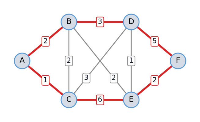
Figure 1:Example network with distances along the edges, and in red the tour A → B → D → F → E → C → A of length 19.
ILO Approach
Model
Decision Variables
if the tour goes from directly to , and 0 otherwise, for with .
Objective
Minimize the length of the tour, .
Constraints
The tour arrives in every city exactly once and leaves every city exactly once:
These constraints are not enough. In Figure 2, every node is entered once and left once, but the red edges form two separate tours, A → B → C → A and D → E → F → D, instead of one tour along all nodes. Such separate tours are called subtours. Their total length is , so a model with only the constraints above would happily return them.
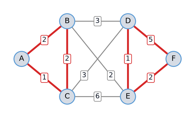
Figure 2:Two subtours (red), A → B → C → A and D → E → F → D. Every node is entered and left exactly once, but this is not one tour.
To prevent subtours, look at a set of nodes and count how many times the tour goes directly from a node in to another node in . A subtour along the nodes of alone does this times, where is the number of nodes in : a tour along nodes has edges. One tour along all nodes, on the other hand, has to leave at some point, and then uses at most edges inside . So we add the subtour elimination constraints
In Figure 2, the set has , so these subtours are no longer feasible.
Complete ILO Model
The price is the number of constraints: a set of nodes has subsets, so there are about subtour elimination constraints. For 50 cities that is constraints, far too many to write down.
Model for the Example
The 10 edges of Figure 1 can each be used in both directions, which gives 20 variables; pairs of nodes without an edge get no variable. With the two directions of each edge grouped, the model is
With 6 nodes there are sets with , so 56 subtour elimination constraints.
Solving the Example in pulp
In practice, the subtour elimination constraints are added only when they are needed, as so-called lazy constraints: solve the model without them, and follow the solution from the start node A until it returns to A. If that tour visits all nodes, it is the optimal tour. If not, it is a subtour: add the subtour elimination constraint for its nodes, and solve again. Usually only a small fraction of all subtour elimination constraints is ever added.
In the code, distance holds each edge once; arc_length adds the reverse
direction, so there is a variable for each of the 20 arcs. The function
follow_tour follows the solution from node to node. A solver computes with
floating-point numbers, so a binary variable can come out as, say, 0.9999999
instead of exactly 1. That is why the code tests var.value() > 0.5 and not
var.value() == 1. As for the algorithms in this lecture, you do not have to be
able to write this code yourself, but you should be able to follow what each line
does and why.
import pulp

distance = {
    ("A", "B"): 2,
    ("A", "C"): 1,
    ("B", "C"): 2,
    ("B", "D"): 3,
    ("B", "E"): 2,
    ("C", "D"): 3,
    ("C", "E"): 6,
    ("D", "E"): 1,
    ("D", "F"): 5,
    ("E", "F"): 2,
}
nodes = ["A", "B", "C", "D", "E", "F"]
# every edge can be used in both directions
reverse = {(j, i): dist for (i, j), dist in distance.items()}
arc_length = distance | reverse

tsp = pulp.LpProblem(name="tsp", sense=pulp.LpMinimize)
travel = {
    (i, j): pulp.LpVariable(name=f"x_{i}_{j}", cat="Binary")
    for (i, j) in arc_length
}
tsp += pulp.lpSum(arc_length[a] * travel[a] for a in arc_length)
for k in nodes:
    arrive = pulp.lpSum(travel[i, j] for (i, j) in arc_length if j == k)
    leave = pulp.lpSum(travel[i, j] for (i, j) in arc_length if i == k)
    tsp += arrive == 1, f"arrive_{k}"
    tsp += leave == 1, f"leave_{k}"


def follow_tour(travel, start):
    """Follow the solution from start until it returns to start."""
    # the node visited after node i
    successor = {i: j for (i, j), var in travel.items() if var.value() > 0.5}
    tour = [start]
    while successor[tour[-1]] != start:
        tour.append(successor[tour[-1]])
    return tour


tsp.solve(pulp.PULP_CBC_CMD(msg=False))
tour = follow_tour(travel, "A")
print(f"length {tsp.objective.value()}: {tour}")
while len(tour) < len(nodes):
    # subtour elimination constraint for the nodes of the subtour
    inside = pulp.lpSum(
        travel[i, j] for (i, j) in arc_length if {i, j} <= set(tour)
    )
    tsp += inside <= len(tour) - 1
    tsp.solve(pulp.PULP_CBC_CMD(msg=False))
    tour = follow_tour(travel, "A")
    print(f"length {tsp.objective.value()}: {tour}")
length 12.0: ['A', 'C']
length 13.0: ['A', 'B', 'C']
length 13.0: ['A', 'B', 'D', 'C']
length 15.0: ['A', 'B', 'E', 'F', 'D', 'C']
In the first solution, the tour from A is A → C → A: going to a neighbor and straight back also enters and leaves every node once. The constraint for is . The second solution contains the subtour A → B → C → A of Figure 2, and the third the subtour A → B → D → C → A. After adding their constraints too, the solver finds one tour of length 15. Only 3 of the 56 subtour elimination constraints were needed. Each time, only the subtour through A gets a constraint; adding one for every subtour in the solution at once usually saves solves. For instances with thousands of cities, specialized solvers use this approach together with many other tricks, but the solution time can still grow very quickly with the number of cities.
Algorithm: Trying All Tours
Is there a dedicated algorithm for the TSP, as Dijkstra’s algorithm is for the shortest path problem? A simple exact algorithm, called brute force, tries every tour:
Start: best length .
For every tour:
Calculate the total distance of the tour.
If it is shorter than the best length so far, it becomes the new best tour.
Fix the start node; then the tour can visit the other nodes in any order. That gives possible tours. For the example with , that is tours, which a computer checks in no time:
import itertools
import math


def edge_length(i, j):
    """Distance between i and j, infinite if there is no edge."""
    return distance.get((i, j), distance.get((j, i), math.inf))


def tour_length(tour):
    """Total distance of a tour (list of nodes) back to its start."""
    return sum(edge_length(i, j) for i, j in zip(tour, tour[1:] + tour[:1]))


start, *others = nodes
best_tour: list[str] = []
best_length = math.inf
n_tours = 0
for order in itertools.permutations(others):
    tour = [start, *order]
    n_tours += 1
    if tour_length(tour) < best_length:
        best_tour, best_length = tour, tour_length(tour)
print(f"checked {n_tours} tours")
print(
    "shortest tour:", " -> ".join(best_tour + [start]), "length", best_length
)
checked 120 tours
shortest tour: A -> B -> E -> F -> D -> C -> A length 15
The running time of this algorithm grows like , and that grows extremely fast. For 20 cities there are tours. Even at a billion tours per second, checking them all takes almost four years, and every extra city multiplies that time by the number of cities. This is not practical for reasonably sized instances.
Can we do better? Unlike for the shortest path and maximum flow problems, no exact algorithm with a polynomial running time is known for the TSP: not via the ILO model, and not via any dedicated algorithm. The next notebook, Complexity and Heuristics, explains what polynomial running time means, why there probably is no such algorithm for the TSP, and then solves this example with a heuristic.
References
Koole, G. (2019). An Introduction to Business Analytics. Chapter 7, “Combinatorial Optimization” (traveling salesman problem).