
An integer linear optimization (ILO) problem is an LO problem with the extra requirement that some or all decision variables take integer values, , or are binary, . (A binary variable is just an integer one with the added constraint .)
In pulp this is a one-word change: set a variable’s cat to "Integer" or "Binary"
instead of the default "Continuous". Everything else about building and solving the
model is the same. Solving it, however, is a different matter: in general ILO is much
harder than LO, as this notebook and Complexity and Heuristics explain.
Learning outcomes
On completion of this notebook, you will be able to:
recognize when a problem needs integer or binary decision variables, and formulate and solve it in pulp;
explain why ILO is generally harder to solve than LO;
explain how branch and bound finds the optimum of an ILO problem;
write any LO problem in the general matrix form;
explain why linearity (but not integrality) is essential for efficient solvability, and how integer variables let you model many other nonlinearities without giving that up.
Why Integer Problems Are Harder¶
Take the bookcase/desk product-mix problem from Linear Optimization and require whole units of and . Its LO optimum was with profit 24.8, not integer. Two things go wrong compared to LO:
the optimal corner is no longer feasible, so the simplex reasoning (“the optimum is at a corner”) does not directly help;
rounding the LO optimum is not enough: rounding both up to violates the oak-panel constraint (), and rounding both down to is feasible but only reaches a profit of 19, well below the true integer optimum. Evaluating nearby integer points tells us little, because finding the true optimum in general needs a systematic search.
Let pulp solve the integer version:
import matplotlib.pyplot as plt
import plotly.graph_objects as go
import pulp
from matplotlib.patches import Rectangle

profit = {"bookcase": 3, "desk": 5}
# resource_use[res][p]: units of resource res per unit of product p
resource_use = {
    "oak panels": {"bookcase": 1, "desk": 3},
    "assembly hours": {"bookcase": 2, "desk": 1},
}
available = {"oak panels": 12, "assembly hours": 10}
products = list(profit)

int_mix = pulp.LpProblem(name="integer_product_mix", sense=pulp.LpMaximize)
dec_vars = {
    p: pulp.LpVariable(name=p, lowBound=0, cat="Integer") for p in products
}
int_mix += pulp.lpSum(profit[p] * dec_vars[p] for p in products)
for res, cap in available.items():
    usage = pulp.lpSum(resource_use[res][p] * dec_vars[p] for p in products)
    int_mix += usage <= cap, res.replace(" ", "_")
int_mix.solve(pulp.PULP_CBC_CMD(msg=False))
print("integer optimum:", {p: dec_vars[p].value() for p in products})
print("optimal profit:", int_mix.objective.value())
integer optimum: {'bookcase': 3.0, 'desk': 3.0}
optimal profit: 24.0
The picture below shows why rounding is unreliable: the LP-relaxation optimum (the star) does not sit on the integer grid, and the nearest lattice points are not necessarily feasible or optimal. The ILO optimum (the diamond) is the best feasible grid point, which can be several steps away from the naive rounding of the relaxation.
Figure 1:Feasible region of the integer product-mix problem with its integer points, the optimum of the LO relaxation (star) and the ILO optimum (diamond). The dashed line contains all points with the optimal integer profit 24: no integer feasible point lies above it, while the LO optimum does. Hover over a point to see its coordinates and profit.
Branch and Bound¶
A common method for solving integer linear optimization (ILO) problems is branch and bound. The basic idea is to start by just ignoring the integer restrictions. More precisely, we allow integer variables to be continuous while retaining all their other bounds and constraints. For example, instead of requiring a binary variable to satisfy , we allow it to take any value between zero and one:
Likewise, instead of requiring , we only require:
This produces the LO relaxation: the same optimization problem, but without the requirement that certain variables must be integers.
The optimal solution to the LO relaxation usually contains non-integer values that should be integers. Such a solution is therefore infeasible for the original ILO problem, but it is still useful in two ways. First, for a maximization problem, it provides an upper bound (UB): the best possible integer solution cannot have a higher objective value than the relaxed solution. Second, it provides a starting point for further search by branching on non-integer variables one by one.
Branching on an LO relaxation that yields an infeasible ILO solution works as follows. Suppose the relaxed solution contains , while should be an integer. We then branch the original root problem into two subproblems based on the LO relaxation of the original problem:
First subproblem: original problem but with extra constraint ;
Second subproblem: original problem but with extra constraint ;
Together, these two subproblems cover all possible integer values of , but neither allows anymore. We then solve the LO relaxation of each subproblem (independently) in the same manner. If either relaxation again yields a non-integer variable that must be integer, we apply the same strategy and branch again, et cetera. To illustrate this, suppose that solving the relaxation for the subproblem with leads to a solution with . We then branch this subproblem again to get one subproblem with constraints and , and one subproblem with and . Indeed, both subproblems still have the previous constraint .
At first sight, this may seem like enumerating all possible integer values. The key difference is that branch and bound uses bounds to avoid exploring subproblems that cannot improve the best integer solution found so far. Hence the name branch and bound.
Any feasible integer solution to the original ILO problem provides a lower bound (LB) for a maximization problem. Along the way, we keep track of the best original ILO solution, called the incumbent. Its objective value is the current best/largest LB. On the other hand, as mentioned before, the LO relaxation of a subproblem is always a UB for the best integer-feasible solution at the subproblem. So if the UB at a subproblem is smaller than the current best LB, we don’t need to branch further on that subproblem, as it will never lead to a better ILO solution. This saves computation time.
Let us formalize this method further. The branch and bound method keeps track of (1) a pool of (sub)problems whose LO relaxation is not solved yet and which may still lead to an optimal solution, and (2) the current best solution with the largest/best LB so far. Initially, this pool contains only the original problem, and the LB is set to . As long as the pool is not empty, choose a (sub)problem from the pool, remove it, and solve its LO relaxation. This solve leads to one of three outcomes:
The found solution is infeasible for the ILO problem, and its objective value is a UB:
If UB largest LB: We eliminate this subproblem (we will not find a better solution here; this can by default not happen for the original problem).
If UB largest LB: Pick a variable from the solution that is non-integer but should be. Branch the (sub)problem on this variable into two new (sub)problems and add them to the pool.
The found solution is feasible for the ILO problem and gives a new LB:
If LB largest LB: Update the new best LB and see whether we can eliminate subproblems that were not eliminated yet. In particular, for all non-eliminated subproblems for which we obtained a UB, check whether their UB largest LB; if so, eliminate the subproblem and remove all its descendants still in the pool.
If LB largest LB: Eliminate this subproblem (nothing to branch further here).
There is no feasible solution for the specific (sub)problem: Eliminate this subproblem as it cannot have an ILO feasible solution.
Keep repeating this procedure until the pool is empty. Once the pool is empty, we are guaranteed that the solution with the current best LB is optimal.
The process can be visualized as a tree. The original problem is the root. Each time we branch, we split one (sub)problem into two child subproblems. The pool contains the subproblems that have not yet been eliminated or solved.
We did not discuss how to choose two things: which decision variable to branch on (since an LO relaxation solution typically has many non-integer variables that should be integer) and which (sub)problem from the pool to pick first. The choice affects performance, and what works best is a research topic on its own and outside the scope of this course. In this course, just make a choice; we always know that in the end we will find the optimal solution.
Let us apply this idea to the integer product-mix problem to illustrate its workings. We number the steps in the order in which we take them:
Step 1: root problem. The LO relaxation has optimum with objective value 24.8. This is a UB, but the solution is not integer in both decision variables and thus infeasible. Just pick a decision variable to branch on. We branch on , which adds the subproblems with and to the pool.
Step 2: left subproblem, the root problem with . Its relaxation has optimum with value 22. This solution is integer, so it is feasible for the ILO problem and thus holds the current best LB of 22. No need to branch further from this subproblem.
Step 3: right subproblem, the root problem with . Its relaxation has optimum with value 24. This is also feasible for the ILO problem, so it improves the best LB to 24, and we can replace the previous best solution with the solution . No need to branch further from this subproblem.
Step 4: left subproblem is suboptimal. Its value of 22 is below the new best LB of 24, so the solution is no longer the best one.
Step 5: optimum. The pool is now empty (no promising (sub)problems left to explore), so we are done, and the current best solution of with profit 24 must be the optimal ILO solution.
The figure below shows these steps as a branch-and-bound tree. Each node is a (sub)problem: its header gives the step in which its LO relaxation is solved, the objective value, and whether that value is a UB or a LB, and the line below gives the relaxation’s optimal solution . The labels on the edges are the constraints added by branching.
Source
# header and body colors per node type, and colors of the status boxes
NODE_COLORS = {
    "UB": ("#5b9bd5", "#d6dce5"),
    "LB": ("#70ad47", "#d9e7cf"),
    "infeasible": ("#e00000", "#fbd5b5"),
}
STATUS_COLORS = {"pruned": "#e00000", "optimum": "#375623"}
EDGE_COLOR = "#5b9bd5"


def draw_bb_tree(
    nodes, edges, status, xlim, ylim, figsize, box_width=3.6, font_size=11
):
    """Draw a branch-and-bound tree.

    nodes: name -> (x, y, header, solution, node type)
    edges: (parent, child, branching constraint) tuples
    status: name -> (text, status type) for a box below the node

    The background is transparent and every text sits on its own box, so
    the figure reads the same in the light and the dark site theme.
    """
    box_height, gap = 0.55, 0.08
    fig, ax = plt.subplots(figsize=figsize, dpi=150)
    fig.patch.set_alpha(0)
    ax.patch.set_alpha(0)
    for parent, child, branch_label in edges:
        x_from, y_from = nodes[parent][:2]
        x_to, y_to = nodes[child][:2]
        y_from -= 1.5 * box_height + gap
        y_to += 0.5 * box_height
        ax.plot([x_from, x_to], [y_from, y_to], color=EDGE_COLOR, lw=1.2)
        ax.text(
            (x_from + x_to) / 2,
            (y_from + y_to) / 2,
            branch_label,
            ha="center",
            va="center",
            fontsize=font_size,
            color="#111827",
            bbox={
                "boxstyle": "round,pad=0.3",
                "facecolor": "white",
                "edgecolor": EDGE_COLOR,
            },
        )
    for node, (x_c, y_c, header, body, node_type) in nodes.items():
        dark, light = NODE_COLORS[node_type]
        boxes = [(header, dark, "white", "bold"), (body, light, "black", "")]
        if node in status:
            text, status_type = status[node]
            boxes.append((text, STATUS_COLORS[status_type], "white", "bold"))
        for row, (text, face, text_color, font_weight) in enumerate(boxes):
            y_row = y_c - row * (box_height + gap)
            ax.add_patch(
                Rectangle(
                    (x_c - box_width / 2, y_row - box_height / 2),
                    box_width,
                    box_height,
                    facecolor=face,
                    edgecolor="none",
                )
            )
            ax.text(
                x_c,
                y_row,
                text,
                ha="center",
                va="center",
                color=text_color,
                fontweight=font_weight or "normal",
                fontsize=font_size,
            )
    ax.set_xlim(*xlim)
    ax.set_ylim(*ylim)
    ax.axis("off")
    plt.show()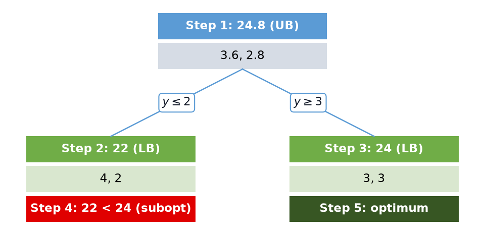
Figure 2:Branch-and-bound tree for the integer product-mix problem (UB = upper bound from the LO relaxation, LB = lower bound from a feasible integer solution, subopt = suboptimal solution).
In this example, we needed only three LO relaxations, rather than checking every possible integer combination. Modern integer-optimization solvers use this basic branch-and-bound idea, often enhanced with additional techniques. More on this later.
The Knapsack Problem¶
Let us now illustrate branch and bound on an archetypical ILO problem called the knapsack problem. We will first give a practical motivation for this problem, then we will model the problem as an ILO problem. The ILO problem will be made concrete for a small example, which is then solved in pulp. We finish with some extensions.
Practical Motivation¶
A transport company has one truck left for tomorrow and more shipment requests than the truck can carry. Each shipment earns a known revenue and has a known weight, and the truck has a maximum load. Which shipments should it accept to earn as much as possible? The same question comes up when choosing which projects to fund from a fixed budget, which pieces to cut from a steel plate, or which items to pack for a trip.
Modeling¶
Problem Definition and Example¶
There are items. Item has a reward and a weight , and the knapsack has a capacity . The problem is to choose a subset of the items with maximum total reward whose total weight does not exceed the capacity.
As an example, take items and capacity :
| item | 1 | 2 | 3 | 4 |
|---|---|---|---|---|
| reward | 15 | 9 | 10 | 5 |
| weight | 1 | 3 | 5 | 4 |
For example, taking items 2 and 3 gives a total reward of and a total weight of , which fits exactly. Adding item 1 as well would give a weight of 9, which does not fit.
Decision Variables¶
For every item we decide whether to take it or not. An item cannot be taken in part, so we use a binary decision variable per item:
Objective¶
Item adds to the reward if it is taken () and nothing if it is not (), so the total reward is summed over all items. We maximize
Constraints¶
In the same way, the total weight of the items taken is , which may not exceed the capacity:
Finally, for all .
Complete ILO Model¶
Solving the Example in pulp¶
The only change from an LO model in pulp is cat="Binary" for the decision variables.
The items are numbered, so we store the data in lists and the variables in a list
take, where take[i] is (Python counts from 0). Printing the model is a
quick way to check that it matches the model above.
# data
reward = [15, 9, 10, 5]
weight = [1, 3, 5, 4]
capacity = 8
n_items = len(reward)

# modeling
knapsack = pulp.LpProblem(name="knapsack", sense=pulp.LpMaximize)
take = [
    pulp.LpVariable(name=f"x_{i + 1}", cat="Binary") for i in range(n_items)
]
knapsack += pulp.lpSum(reward[i] * take[i] for i in range(n_items))
total_weight = pulp.lpSum(weight[i] * take[i] for i in range(n_items))
knapsack += total_weight <= capacity, "capacity"
print(knapsack)

# solve and print solution
knapsack.solve(pulp.PULP_CBC_CMD(msg=False))
print("take items:", [i + 1 for i in range(n_items) if take[i].value() == 1])
print("total reward:", knapsack.objective.value())
knapsack:
MAXIMIZE
15*x_1 + 9*x_2 + 10*x_3 + 5*x_4 + 0.0
SUBJECT TO
capacity: x_1 + 3 x_2 + 5 x_3 + 4 x_4 <= 8
VARIABLES
0 <= x_1 <= 1 Integer
0 <= x_2 <= 1 Integer
0 <= x_3 <= 1 Integer
0 <= x_4 <= 1 Integer
take items: [1, 2, 4]
total reward: 29.0
The optimal choice is items 1, 2 and 4, with a total reward of 29 and a total weight of 8.
Extensions¶
Several Copies per Item¶
If up to copies of item are available, becomes the number of copies taken: replace by , an integer variable with upper bound . The objective and the capacity constraint stay the same.
Several Knapsacks¶
With several knapsacks (for example, several trucks) with capacities , the decision is which item goes into which knapsack. Use a binary that is 1 if item goes into knapsack , require so that every item is used at most once, and give every knapsack its own capacity constraint .
Branch and Bound for the Knapsack Example¶
We now solve the same example by hand with branch and bound.
Solving the LO Relaxation¶
Every step of branch and bound solves an LO relaxation, so we first need to know how to do that. For the knapsack problem this turns out to be easy, and no LO solver is needed.
In the LO relaxation, becomes : we may take any fraction of an item, and a fraction of item gives reward and uses capacity . Each unit of capacity should then go to the item that gives the most reward per unit of weight. So we sort the items in decreasing order of their reward-to-weight ratio and fill the knapsack in that order, taking each item completely as long as it fits. The first item that no longer fits completely is taken for the fraction that fills the remaining capacity, and all later items are left out. As a result, at most one variable in the optimal solution of the LO relaxation is fractional.
For our example, the ratios are , , and , so the items are already in decreasing order of ratio. Filling the knapsack in that order goes as follows:
| item | ratio | weight | fraction taken | capacity left |
|---|---|---|---|---|
| 1 | 15 | 1 | 1 | 7 |
| 2 | 3 | 3 | 1 | 4 |
| 3 | 2 | 5 | 4/5 | 0 |
| 4 | 1.25 | 4 | 0 | 0 |
Items 1 and 2 fit completely. Item 3 does not: only 4 of its weight of 5 fits, so we take a fraction of it, and there is no capacity left for item 4. The optimal solution of the LO relaxation is therefore with objective value .
In branch and bound, some variables are fixed to 0 or 1 in a subproblem. The same rule then still applies: items fixed to 1 are packed first, items fixed to 0 are left out, and the remaining items fill the remaining capacity in decreasing order of ratio. If the items fixed to 1 already exceed the capacity, the subproblem is infeasible.
Branch and Bound Steps¶
With the LO relaxation in hand, we solve our example with branch and bound. Since the LO relaxation has at most one fractional variable, there is only one variable to branch on in each step, and branching on a binary variable means fixing it to 0 in one subproblem and to 1 in the other. We use the same step numbering as before:
Step 1: root problem. The LO relaxation has optimum with value 32, a UB. We branch on .
Step 2: subproblem . Without item 3, items 1, 2 and 4 fit exactly: the relaxation has optimum with value 29. This solution is integer, so it is feasible for the ILO problem and gives the current best LB of 29. No need to branch further from this subproblem.
Step 3: subproblem . Item 3 uses 5 of the capacity, item 1 then fits, and of item 2 fills the rest: optimum with value 31. This UB is larger than the best LB of 29, so this subproblem may still contain a better solution. We branch on .
Step 4: subproblem , . Items 3 and 1 fit, and half of item 4 fills the rest: optimum with value 27.5, a UB.
Step 5: eliminate. The UB of 27.5 is below the best LB of 29, so this subproblem cannot contain a better solution and we eliminate it without branching.
Step 6: subproblem , . Items 3 and 2 use the full capacity, so item 1 no longer fits: optimum with value 19. This solution is integer and thus a LB.
Step 7: suboptimal. The LB of 19 is below the best LB of 29.
Step 8: optimum. The pool is now empty, so the best solution found, with reward 29 from step 2, is optimal.
The figure below shows the branch-and-bound tree.
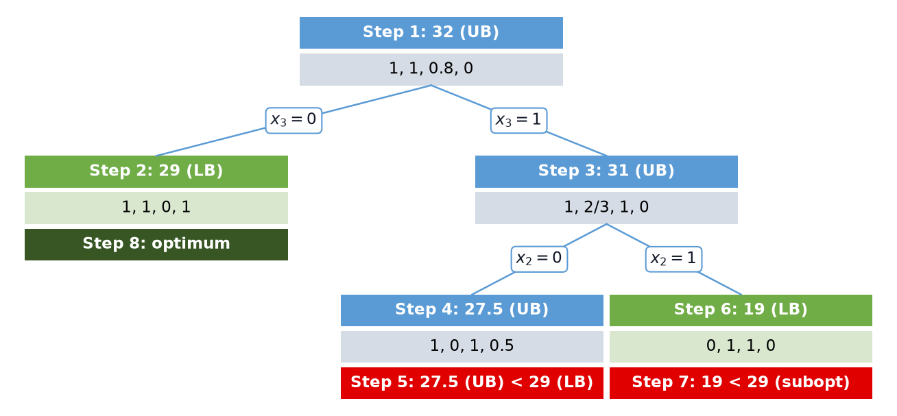
Figure 3:Branch-and-bound tree for the knapsack example (UB = upper bound from the LO relaxation, LB = lower bound from a feasible integer solution, subopt = suboptimal solution).
General Formulation¶
Having now seen both LO and ILO in action, we can step back and write down the general form both fit into. An LO problem with decision variables and constraints is
or in matrix notation , with column vectors of length , a column vector of length , and an matrix.
This one form covers more than it seems. Every other case can be rewritten into it:
minimization: ;
“” constraints: ;
“” constraints: and ;
free (unrestricted) variables: replace by with .
Why Linearity Matters, and What Integrality Buys Back¶
Linearity is what makes LO efficiently solvable: written in the general form above, the feasible region is a convex polyhedron, an optimum sits at a corner, and a local optimum is automatically global. As soon as the objective or a constraint is nonlinear, both of those break:
Nonlinear objective. Maximize subject to , . The optimum is , in the interior of an edge, not at a corner.
Nonlinear constraint. Maximize subject to , , . The feasible set is two line segments meeting at the origin (either or ). It has two local optima, and ; you cannot be sure which is global without checking both. More generally, the simplex reasoning from Linear Optimization breaks down whenever the feasible region is not a convex polyhedron: you are not sure you have found the best solution until you have checked every local optimum, which is usually intractable.
Nonlinear optimization therefore needs slower, less reliable algorithms. But there is a large and useful middle ground: integer constraints. On the one hand, requiring is itself a nonlinear constraint, and it does make a problem harder to solve, as branch and bound’s extra work above shows. On the other hand, unlike general nonlinearities, it is not intractably so, and many other nonlinearities (an either/or choice, a fixed cost that applies only when an activity is used, a “this constraint holds only if...” condition) can be expressed with integer (usually binary) variables and otherwise-linear constraints, and then solved with branch and bound. That is why so much modeling effort goes into casting a problem as ILO, and why it is worth treating as its own class rather than lumping it in with general nonlinear optimization. Set Covering and Shift Scheduling and Machine Scheduling show many of those tricks in practice.
References¶
Koole, G. (2019). An Introduction to Business Analytics. §6.4 “Integer Problems.”