
The smaller exercises embedded in Introduction, Linear Optimization, and Integer Optimization check what you just read. This notebook collects the larger exercises for Lecture 8: independent problems worth more time, starting with a set of homework exercises, followed by further exercises.
Homework Exercises
Solution to Exercise 1 #
a. Let and be the number of units produced of product 1 and 2, respectively. Then the LO is
b. The figure below shows the feasible region. Shifting the objective line up (increasing ) as far as possible, it last touches the feasible region where the lines and cross. Substituting in gives : the optimal solution is with objective value 7.5.
Figure 1:Solution of Exercise 1, part b: the feasible region of part a, with the objective line through the optimum . Hover over a corner point to see its objective value.
c. Only has to be integer; may still take any value. We use branch and bound. The LO relaxation is the problem of part b, with optimum and UB 7.5. Since is not integer, we branch on :
: the LO optimum is with value 7. Here is integer, so this is a feasible solution and gives LB 7. It is also the only optimal solution of this subproblem, since and .
: now , and the labor constraint gives , so the objective is at most . The LO optimum is therefore with value 7, again with integer , and no other point of this subproblem reaches 7.
Both subproblems are solved and the pool is empty, so the optimal value is 7, and it is reached in both subproblems. The optimal solutions are and . The figure below shows the same result graphically: with integer , the feasible solutions are the horizontal line segments, and the objective line touches them in exactly these two points.
Figure 2:Solution of Exercise 1, part c: with integer and continuous, the feasible solutions lie on the horizontal segments. The objective line touches them in and . Hover over a segment or point for its objective value.
d. Let binary if the exchange is used, 0 otherwise. The ILO becomes
Case is solved in part b, objective 7.5. For , the labor constraint becomes , and the corner of the feasible region moves to where meets (labor used: ), giving objective . Since , it is optimal to use the exchange.
Solution to Exercise 2 #
a. Let and be the number of units produced of bread types A and B. Then the LO is
b. The figure below shows the feasible region. Shifting the objective line up as far as possible, it last touches the feasible region where the lines and cross. Subtracting the first equation from the second gives , and then : the optimal solution is with objective value 6.25.
Figure 3:Solution of Exercise 2, part b: the feasible region of part a, with the objective line through the optimum . Hover over a corner point to see its objective value.
c. The objective function is .
i. : since A earns no profit, it is optimal to bake as much B as possible. The flour constraint limits this to 5 units of B, so .
ii. The point lies on the flour constraint line and satisfies the yeast constraint (), so it lies on the edge of the feasible region between and . Choosing the objective line parallel to this edge, e.g. , makes every point on the edge optimal, including .
d. Let nonnegative be the less profitable version of that is unrestricted from above, and restrict itself by the upper bound 2. The LO becomes
Since and use the same resources and is more profitable, an optimal solution only has if is at its upper bound 2. There are two cases (see the figure below):
: then the model of part a applies with the extra constraint . Drawing this constraint in the figure of part b shows that the optimum is now , with objective value .
: then , and the LO reduces to
In the plane, the objective line reaches furthest where crosses the axis , so the optimum is with objective value 6. So a positive does not pay off.
Both cases lead to the same solution, so with profit 6 is optimal: bake 2 units of A and 3 units of B.
Figure 4:Solution of Exercise 2, part d: the two cases. Left: , the region of part b with added. Right: , so , and the remaining problem in and . Hover over a corner point to see its objective value.
Solution to Exercise 3 #
a. Number the items 1-4 and let if item is taken, 0 otherwise. The ILO is
All rewards are positive, so an optimal solution leaves no room for another item. Each item weighs at least 2 kg and items 3 and 4 together already weigh 8 kg, so the solutions that use the capacity as much as possible are items (8 kg, reward 12), items (8 kg, reward 9) and items (8 kg, reward 13). The optimal solution is with reward 13.
b. As in Integer Optimization, fill the knapsack in decreasing order of the reward-to-weight ratios, which are euro/kg for items 1-4. The order is 3, 1, 4, 2. Items 3 and 1 fit completely (total weight ), leaving 3 kg for item 4 (weight 4), i.e. a fraction of it. The optimal solution of the LO relaxation is with objective value .
c. We follow the branch and bound procedure and solve every LO relaxation as in part b, packing the items fixed to 1 first. The order in which subproblems are picked from the pool is a choice. Here we solve both subproblems of the root first and then continue depth first: we always pick the most recently created subproblem, with the branch before .
Step 1: root problem. From part b: with value 14.75, a UB. We branch on .
Step 2: . Items 3, 1 and 2 all fit (8 kg): with value 12. This solution is integer, so it gives the current best LB of 12.
Step 3: . Item 4 uses 4 kg; item 3 then fits and half of item 1 fills the last kg: with value 14.5. This UB is larger than 12, so we branch on .
Step 4: , . Items 4 and 3 fit, and half of item 2 fills the last kg: with value 13.5, a UB larger than 12. We branch on .
Step 5: , , . Items 4 and 3: with value 13. This solution is integer and improves the best LB to 13.
Step 6: suboptimal. The solution of step 2 has value .
Step 7: , , . Items 4 and 2 use 6 kg, and of item 3 fills the rest: with value 12, a UB.
Step 8: eliminate. The UB of 12 is below the best LB of 13.
Step 9: , . Items 4 and 1 use 6 kg, and of item 3 fills the rest: with value 14, a UB larger than 13. We branch on .
Step 10: , , . Items 4 and 1, and item 2 still fits: with value 9, an integer solution and thus a LB.
Step 11: suboptimal. The LB of 9 is below the best LB of 13.
Step 12: , , . The items fixed to 1 weigh kg, so this subproblem is infeasible and is eliminated.
Step 13: optimum. The pool is empty, so the best solution found, with reward 13 from step 5, is optimal. This matches part a.
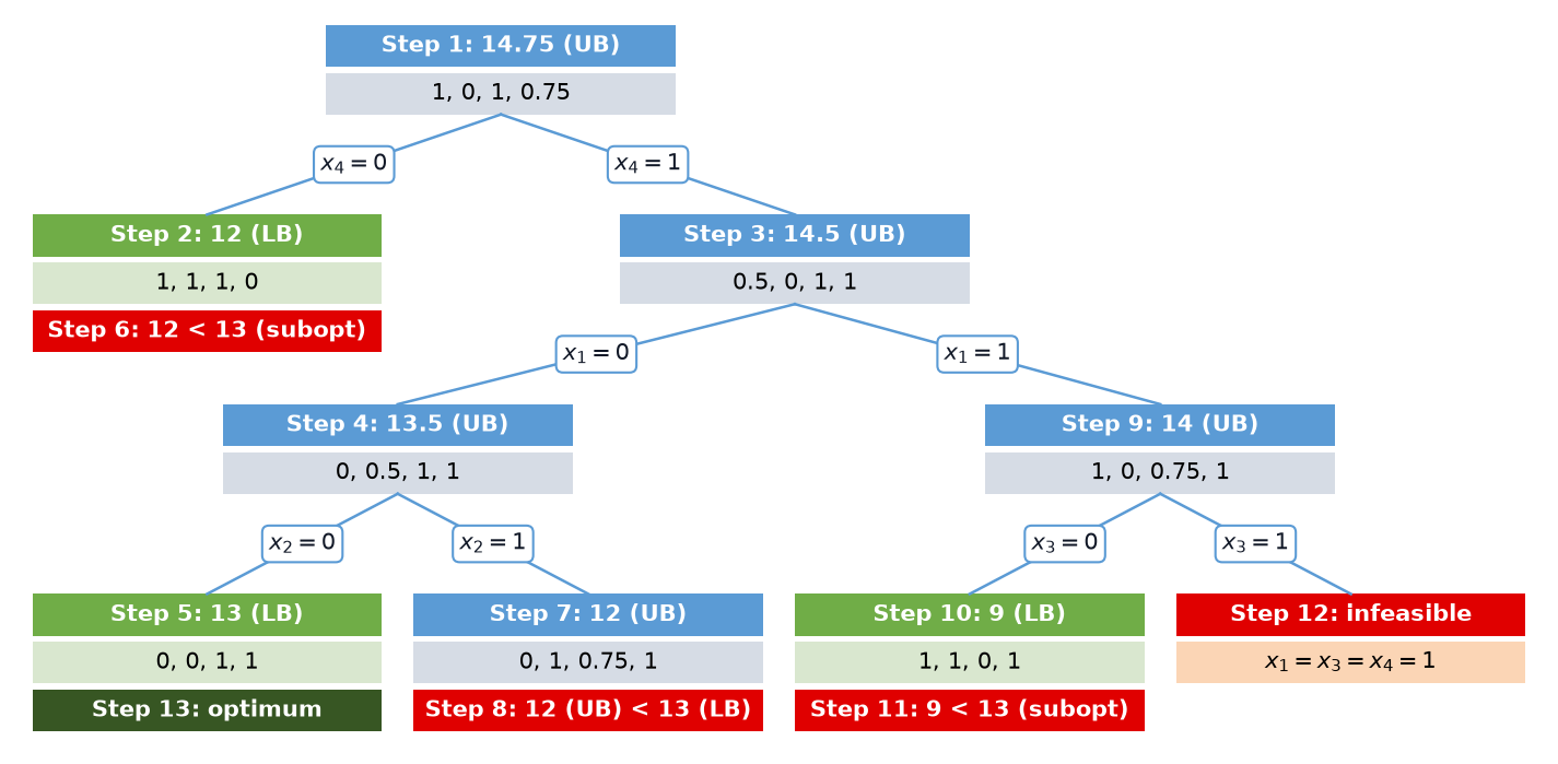
Figure 5:Solution of Exercise 3, part c: branch-and-bound tree (UB = upper bound from the LO relaxation, LB = lower bound from a feasible integer solution, subopt = suboptimal solution). The infeasible subproblem of step 12 has no solution; its second line shows the variables fixed to 1.
d. Add the constraint to the model of part a. An extra constraint can only make the feasible region smaller, so the optimal value cannot increase. The solution from part c uses volume , so it is still feasible, and with reward 13 it is still optimal.
Solution to Exercise 4 #
a. Let and be the number of units produced of product 1 and 2. Then
b. The figure below shows the feasible region. Shifting the objective line up as far as possible, it last touches the feasible region where the lines and cross. From the first line, ; substituting in the second gives , so and , with objective value .
Figure 6:Solution of Exercise 4, part b: the feasible region of part a, with the objective line through the LO optimum and the feasible integer points used in part c. Hover over a point to see its objective value.
c. Add the constraints . The LO optimum of part b is an upper bound: no integer solution has a value above . With and integer, the value is integer too, so it is at most 5. The point is feasible ( and ) and has value 5, so it reaches this bound and is optimal. In the figure: shifting the objective line down from the LO optimum, is the first feasible integer point it reaches.
d. Constraint becomes . The LO optimum is now where meets : , , objective value 6. Since this solution is already integer, it is also optimal for the integer case. The additional revenue compared to part c is .
Solution to Exercise 5 #
a. Let and be the number of chairs and tables made. The objective adds up profit[p] * make[p], and the loop creates one constraint per resource, with use[res][p] as coefficients and the resource name as constraint name:
b. The corner points of the feasible region are with profit 0, with profit 16, with profit 24, and the point where both resource constraints are met exactly. Subtracting from gives , so this point is with profit : the optimum. pulp prints the values as floats:
Optimal
{'chair': 2.0, 'table': 3.0}
26.0
c. (i) With >=, both constraints say “at least”: the feasible region contains points with arbitrarily many chairs and tables, and since we maximize profit, the problem is unbounded. The first line becomes Unbounded: there is no optimal solution.
(ii) Minimizing the profit: making nothing is feasible, and the profit cannot be negative, since both variables are at least 0 and both profits are positive. The first line is still Optimal, now with both values 0 and objective value 0.
Further Exercises
These further exercises test your knowledge, your pulp skills, and include more homework-style questions: some from the book, some that need pulp (not possible on the exam).