Lecture 9: Exercises - Simulation and Optimization: Lecture Notes

The smaller exercises embedded in Transportation and Transshipment, Set Covering and Shift Scheduling, and Machine Scheduling check what you just read. This notebook collects the homework exercises for Lecture 9: independent problems worth more time.

Homework Exercises¶

Exercise 1¶

Exercise 1

A manager has to allocate 3 workers to 2 tasks: how many hours each worker spends on each task. The total working hours available for the workers are 20, 20, and 5, respectively. The tasks require 30 and 40 effective working hours, respectively. The effective working hour rate indicates how many effective hours a specific worker contributes to a specific task per hour worked:

Worker \ Task	1	2
1	0.1	10
2	2	2
3	5	8

For example, each hour worked by worker 1 on task 2 gives 10 effective working hours. The manager wants to minimize the total hours worked while ensuring that (i) both tasks are done, and (ii) no worker’s total hours are exceeded.

a. Model this as a linear optimization problem.

b. Give a restriction that ensures worker 1 works at most 5 hours on task 2.

c. Now only one worker may work on task 1. Model this as an integer linear optimization problem.

d. The restriction from part c is lifted again. Instead, if workers 2 and 3 both work on task 1, 10 extra effective working hours are required for task 1 (due to coordination overhead). Model this as an integer linear optimization problem.

Solution to Exercise 1 #

a. Define $x_{ij}$ as the decision variable for the number of hours worker $i$ works on task $j$ , for $i = 1, 2, 3$ and $j = 1, 2$ . The LO is

\begin{aligned} \min \quad & \sum_{i=1}^{3} \sum_{j=1}^{2} x_{ij} \\ \text{s.t.} \quad & x_{11} + x_{12} \le 20 & \text{(hours worker 1)} \\ & x_{21} + x_{22} \le 20 & \text{(hours worker 2)} \\ & x_{31} + x_{32} \le 5 & \text{(hours worker 3)} \\ & 0.1x_{11} + 2x_{21} + 5x_{31} \ge 30 & \text{(task 1)} \quad (\ast) \\ & 10x_{12} + 2x_{22} + 8x_{32} \ge 40 & \text{(task 2)} \\ & x_{ij} \ge 0, \quad i = 1, 2, 3,\ j = 1, 2. \end{aligned}

(1)

The objective is the total number of hours worked. The first three constraints make sure no worker works more than their available hours, and the last two that each task gets at least its required effective hours.

b. The restriction is $x_{12} \le 5$ .

c. Define $z_i$ as a binary decision variable that is 1 if worker $i$ works on task 1, and 0 otherwise, for $i = 1, 2, 3$ . Let $M$ be a big constant, for example $M = 1000$ (any $M \ge 20$ works, since no worker has more than 20 hours). Add to the LO of part a the constraints

\begin{aligned} & x_{i1} \le M z_i, \quad i = 1, 2, 3 & (\ast\ast) \\ & z_1 + z_2 + z_3 = 1 \\ & z_i \in \{0, 1\}, \quad i = 1, 2, 3. & (\ast\ast\ast) \end{aligned}

(2)

Constraint $(\ast\ast)$ gives $z_i$ its meaning: if worker $i$ works on task 1 ( $x_{i1} > 0$ ), then $z_i$ must be 1, and if $z_i = 0$ then $x_{i1} = 0$ . The second constraint then allows exactly one worker on task 1.

d. Start from the LO of part a. Define $q$ as a binary decision variable that is 1 if workers 2 and 3 both work on task 1, and 0 otherwise. To require 10 extra effective hours for task 1 when $q = 1$ , replace constraint $(\ast)$ by

0.1x_{11} + 2x_{21} + 5x_{31} \ge 30 + 10q.

(3)

Now we make sure that $q$ gets the value of its definition. First, add the constraints $(\ast\ast)$ and $(\ast\ast\ast)$ of part c for $i = 2, 3$ (but not $z_1 + z_2 + z_3 = 1$ ), so that $z_2$ and $z_3$ have the same meaning as in part c. Then add

\begin{aligned} & q \ge z_2 + z_3 - 1 \\ & q \in \{0, 1\}. \end{aligned}

(4)

If $z_2 = z_3 = 1$ , this forces $q = 1$ . Otherwise the constraint allows $q = 0$ , and since a larger $q$ only requires more work, minimizing the total hours sets $q = 0$ (“less work”). For the same reason the optimizer never sets $z_i = 1$ for a worker who does not work on task 1.

Exercise 2¶

Exercise 2

A hospital has 4 candidate locations, A, B, C, D, to place an ambulance so as to cover 5 cities, numbered 1-5. The travel time (minutes) from each location to each city is:

Location \ City	1	2	3	4	5
A	3	4	8	10	8
B	8	5	4	10	12
C	6	9	8	7	3
D	8	7	4	2	6

At each location, at most one ambulance can be placed. The hospital wants to minimize the number of ambulances placed while ensuring every city is reachable within 5 minutes or less from at least one location with a placed ambulance.

a. Describe how this problem is a set cover problem: give the universe and the sets.

b. Model the problem as an integer linear optimization problem.

c. Using part b, is placing ambulances at locations A and C only a feasible allocation? Motivate your answer.

d. Give the optimal solution and motivate why it is optimal.

import matplotlib.pyplot as plt
from matplotlib.patches import Circle

# Static figure for the light and the dark site theme: transparent
# background, and every text sits on its own box. At 120 dpi a 10 pt font is
# about 16 px, the size of the page text, when the figure is shown at its
# natural width.
FONT_SIZE = 10
TEXT_COLOR = "#111827"
EDGE_COLOR = "#888888"
LABEL_BOX = {
    "boxstyle": "round,pad=0.25",
    "facecolor": "white",
    "edgecolor": EDGE_COLOR,
}
# name -> (x, y, supply or demand)
net_sources = {
    "S1": (0.0, 2.6, 30),
    "S2": (0.0, 1.3, 10),
    "S3": (0.0, 0.0, 10),
}
net_destinations = {"D1": (3.0, 2.0, 25), "D2": (3.0, 0.6, 25)}
arc_cost = {
    ("S1", "D1"): 1,
    ("S1", "D2"): 2,
    ("S2", "D1"): 3,
    ("S2", "D2"): 5,
    ("S3", "D1"): 5,
    ("S3", "D2"): 3,
}
node_radius = 0.24
# fraction of the way along an arc where its cost label sits
label_pos = 0.27

fig, ax = plt.subplots(figsize=(4.6, 2.7), dpi=120)
fig.patch.set_alpha(0)
ax.patch.set_alpha(0)
for (src, dst), arc_label in arc_cost.items():
    x_src, y_src, _ = net_sources[src]
    x_dst, y_dst, _ = net_destinations[dst]
    ax.annotate(
        "",
        xy=(x_dst, y_dst),
        xytext=(x_src, y_src),
        arrowprops={
            "arrowstyle": "-|>",
            "color": EDGE_COLOR,
            "lw": 1.3,
            "shrinkA": 15,
            "shrinkB": 15,
        },
    )
    ax.text(
        x_src + label_pos * (x_dst - x_src),
        y_src + label_pos * (y_dst - y_src),
        str(arc_label),
        ha="center",
        va="center",
        fontsize=FONT_SIZE,
        color=TEXT_COLOR,
        bbox=LABEL_BOX,
    )
node_groups = [
    (net_sources, "#2ca02c", -1, "supply"),
    (net_destinations, "#1f77b4", 1, "demand"),
]
for nodes, face, side, word in node_groups:
    for name, (x_node, y_node, amount) in nodes.items():
        disc = Circle((x_node, y_node), node_radius, facecolor=face, lw=0)
        ax.add_patch(disc)
        ax.text(
            x_node,
            y_node,
            name,
            ha="center",
            va="center",
            fontsize=FONT_SIZE,
            color="white",
            fontweight="bold",
        )
        ax.text(
            x_node + side * (node_radius + 0.12),
            y_node,
            f"{word} {amount}",
            ha="right" if side < 0 else "left",
            va="center",
            fontsize=FONT_SIZE,
            color=TEXT_COLOR,
            bbox=LABEL_BOX,
        )
ax.set_xlim(-1.25, 4.25)
ax.set_ylim(-0.3, 2.9)
ax.set_aspect("equal")
ax.axis("off")
plt.show()

Exercise 3¶

Exercise 3

Consider the transportation problem in the figure below. Three sources S1, S2 and S3 with their supply are on the left, two destinations D1 and D2 with their demand on the right, and the label on each arc is the cost per unit shipped over it.

Figure 1:Transportation network of Exercise 3, with the cost per unit on each arc.

a. Give the LO formulation of this problem.

b. Extend this formulation so that at most 3 arcs are used in total.

A number of first-year students need to be assigned to rooms in student dormitories: there are $n$ students and $n$ rooms, and each student ranks the rooms.

c. Formulate this as a transportation problem: give the sources, destinations, and a reasonable cost function.

d. Change the formulation so it can be used to decide whether it is possible to accommodate everyone according to their top-3 preferences. Explain your answer.

Solution to Exercise 3 #

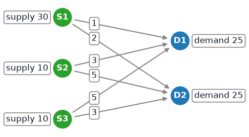
a. Define $x_{ij}$ as the decision variable for the quantity transported from source S $i$ to destination D $j$ , for $i = 1, 2, 3$ and $j = 1, 2$ . The LO is

\begin{aligned} \min \quad & x_{11} + 2x_{12} + 3x_{21} + 5x_{22} + 5x_{31} + 3x_{32} \\ \text{s.t.} \quad & x_{11} + x_{12} \le 30 & \text{(supply S1)} \\ & x_{21} + x_{22} \le 10 & \text{(supply S2)} \\ & x_{31} + x_{32} \le 10 & \text{(supply S3)} \\ & x_{11} + x_{21} + x_{31} \ge 25 & \text{(demand D1)} \\ & x_{12} + x_{22} + x_{32} \ge 25 & \text{(demand D2)} \\ & x_{ij} \ge 0, \quad i = 1, 2, 3,\ j = 1, 2. \end{aligned}

(6)

The inequality signs may be replaced by equality signs here: total supply equals total demand ( $30 + 10 + 10 = 25 + 25$ ), so the only way to meet all demand is to ship every unit of supply, and then every constraint holds with equality.

b. Define $z_{ij}$ as a binary decision variable that is 1 if arc $(i, j)$ is used, and 0 otherwise, for $i = 1, 2, 3$ and $j = 1, 2$ . Let $M$ be a big constant, for example $M = 1000$ (any $M \ge 25$ works, since no arc carries more than a demand of 25). Add to the LO of part a

\begin{aligned} & x_{ij} \le M z_{ij}, \quad i = 1, 2, 3,\ j = 1, 2 \\ & \sum_{i=1}^{3} \sum_{j=1}^{2} z_{ij} \le 3 \\ & z_{ij} \in \{0, 1\}, \quad i = 1, 2, 3,\ j = 1, 2. \end{aligned}

(7)

The first constraint gives $z_{ij}$ its meaning: an arc that carries goods has $z_{ij} = 1$ . The second then limits the number of arcs used to 3.

This model is correct, but this particular instance has no feasible solution. As shown in part a, every unit of supply must be shipped. S1 has 30 units, more than either destination needs, so it uses both of its arcs, and S2 and S3 each use at least one arc: at least 4 arcs are needed.

c. The sources are the students and the destinations are the rooms. The supply of every source and the demand of every destination is 1. The cost from student $i$ to room $j$ is the rank student $i$ gives room $j$ : if student $i$ ranks room $j$ as number $r$ , the cost of arc $(i, j)$ is $r$ , so a more preferred room costs less. Since all supplies and demands are integer, the LO optimum is integer, so it really assigns each student to one room.

d. In the formulation of part c, redefine the cost of arc $(i, j)$ as 0 if room $j$ is in student $i$ ’s top 3, and 1 otherwise. Then the total cost of an assignment is the number of students who do not get a top-3 room. Solve the transportation problem: if the minimal total cost is 0, the solution is an assignment in which every student gets a top-3 room. If it is positive, no such assignment exists, since any such assignment would have cost 0.

Exercise 4¶

Solution to Exercise 4 #

a. Any choice of 2 sets is optimal. No single set covers $U$ (each set misses one element), so at least 2 sets are needed. Each set misses a different element, so any 2 sets together cover $U$ .

b. Define $x_i$ as a binary decision variable that is 1 if set $S_i$ is chosen, and 0 otherwise, for $i = 1, 2, 3, 4$ . The ILO is

\begin{aligned} \min \quad & x_1 + x_2 + x_3 + x_4 \\ \text{s.t.} \quad & x_1 + x_2 + x_3 \ge 1 & \text{(cover A)} \\ & x_1 + x_2 + x_4 \ge 1 & \text{(cover B)} \\ & x_1 + x_3 + x_4 \ge 1 & \text{(cover C)} \\ & x_2 + x_3 + x_4 \ge 1 & \text{(cover D)} \\ & x_i \in \{0, 1\}, \quad i = 1, 2, 3, 4. \end{aligned}

(8)

c. The LO relaxation is the model of part b with $x_i \in \{0, 1\}$ replaced by $0 \le x_i \le 1$ , for $i = 1, 2, 3, 4$ . An optimal solution is $x_i = \tfrac{1}{3}$ for all $i$ , with objective value $\tfrac{4}{3}$ : it satisfies every cover constraint with equality. No solution does better, since adding the four cover constraints gives $3(x_1 + x_2 + x_3 + x_4) \ge 4$ .

d. Now $x_i \in \{0, 1, 2, \dots\}$ is the number of times set $S_i$ is chosen, and the covering constraints are

\begin{aligned} & x_1 + x_2 + x_3 \ge 3 & \text{(cover A)} \\ & x_1 + x_2 + x_4 \ge 4 & \text{(cover B)} \\ & x_1 + x_3 + x_4 \ge 5 & \text{(cover C)} \\ & x_2 + x_3 + x_4 \ge 6 & \text{(cover D)}. \end{aligned}

(9)

Adding these four constraints gives $3(x_1 + x_2 + x_3 + x_4) \ge 18$ , so the objective value is at least 6. By trial and error, we find the solution $x = (0, 1, 2, 3)$ , which satisfies every constraint (with equality: $0 + 1 + 2 = 3$ , $0 + 1 + 3 = 4$ , $0 + 2 + 3 = 5$ , $1 + 2 + 3 = 6$ ) and has objective value 6. So it is optimal.

Exercise 5¶

Exercise 5

For a classroom assignment, couples need to be formed among 6 students, numbered 1 to 6. Each student lists the students they are willing to work with:

student	1	2	3	4	5	6
willing to work with	2, 3, 4	1, 3, 4	1, 2, 5	2, 6	3, 6	1

A couple can only be formed if both students listed each other. Each student can be part of at most one couple, but not every student needs to be paired.

a. Which couples can be formed?

b. Formulate an integer linear optimization model that maximizes the number of couples formed.

c. Give an optimal solution and motivate why it is optimal.

Solution to Exercise 5 #

a. A couple $\{i, j\}$ can be formed if $j$ is on $i$ ’s list and $i$ is on $j$ ’s list. This gives the couples $\{1, 2\}$ , $\{1, 3\}$ , $\{2, 3\}$ , $\{2, 4\}$ and $\{3, 5\}$ . For example, student 1 lists student 4, but student 4 does not list student 1, so $\{1, 4\}$ cannot be formed. Student 6 cannot be part of any couple.

b. The couple $\{i, j\}$ is the same as the couple $\{j, i\}$ . To have only one decision variable per couple, we use variables $x_{ij}$ with $i < j$ only; this breaks the symmetry between $x_{ij}$ and $x_{ji}$ . Define $x_{ij}$ as a binary decision variable that is 1 if the couple of students $i$ and $j$ is formed, and 0 otherwise, for the couples $\{i, j\}$ with $i < j$ from part a. A couple that cannot be formed gets no variable. The ILO is

\begin{aligned} \max \quad & x_{12} + x_{13} + x_{23} + x_{24} + x_{35} \\ \text{s.t.} \quad & x_{12} + x_{13} \le 1 & \text{(student 1)} \\ & x_{12} + x_{23} + x_{24} \le 1 & \text{(student 2)} \\ & x_{13} + x_{23} + x_{35} \le 1 & \text{(student 3)} \\ & x_{24} \le 1 & \text{(student 4)} \\ & x_{35} \le 1 & \text{(student 5)} \\ & x_{12}, x_{13}, x_{23}, x_{24}, x_{35} \in \{0, 1\}. \end{aligned}

(10)

The objective counts the couples formed. The constraint for student $k$ sums the variables of all couples that contain $k$ , whether $k$ is the first index ( $x_{kj}$ ) or the second ( $x_{ik}$ ), so every student is in at most one couple. The constraints for students 4 and 5 already follow from the binary constraints, and student 6 needs no constraint, since no variable contains student 6.

In general, with $e_{ij} = 1$ if students $i$ and $j$ listed each other (and 0 otherwise), the model is to maximize $\sum_{i<j} x_{ij}$ subject to $x_{ij} \le e_{ij}$ for $i < j$ , and $\sum_{j < k} x_{jk} + \sum_{j > k} x_{kj} \le 1$ for every student $k$ , with $x_{ij} \in \{0, 1\}$ .

c. An optimal solution is $x_{24} = x_{35} = 1$ and all other variables 0: the couples $\{2, 4\}$ and $\{3, 5\}$ , which is feasible since no student is in both. It is optimal because student 6 cannot be paired, so at most 5 students are in a couple, and 5 students form at most 2 couples. (Another optimal solution is $x_{12} = x_{35} = 1$ .)

Exercise 6¶

Exercise 6

A company ships a product from two warehouses, A and B, to three customers, C1, C2 and C3. The supply of each warehouse, the demand of each customer and the transport cost per unit are given in the code below. The transportation model is

\begin{aligned} \min \quad & \sum_{i} \sum_{j} c_{ij} x_{ij} \\ \text{s.t.} \quad & \sum_{j} x_{ij} \le a_i \text{ for every warehouse } i \\ & \sum_{i} x_{ij} \ge b_j \text{ for every customer } j \\ & x_{ij} \ge 0 \text{ for all } i, j, \end{aligned}

(11)

with $x_{ij}$ the number of units shipped from warehouse $i$ to customer $j$ , $c_{ij}$ the cost per unit, $a_i$ the supply and $b_j$ the demand.

a. Complete the code by replacing each ..., so that it solves this model and prints the status, the positive shipments and the total cost.

import pulp

supply = {"A": 60, "B": 45}
demand = {"C1": 20, "C2": 25, "C3": 15}
cost = {
    ("A", "C1"): 2,
    ("A", "C2"): 4,
    ("A", "C3"): 5,
    ("B", "C1"): 3,
    ("B", "C2"): 1,
    ("B", "C3"): 2,
}

transport = pulp.LpProblem(name="transportation", sense=...)
ship = {
    (i, j): ... for (i, j) in cost
}

transport += ...
for i, cap in supply.items():
    shipped = ...
    transport += ..., f"supply_{i}"
for j, need in demand.items():
    received = ...
    transport += ..., f"demand_{j}"

transport.solve(...)
print(pulp.LpStatus[transport.status])
for (i, j), var in ship.items():
    if var.value() > 0:
        print(i, "->", j, var.value())
print("total cost:", transport.objective.value())

b. Warehouse B can ship at most 10 units to customer C2. Change the code of part a to take this into account.

c. Start again from the code of part a. Using a warehouse costs a fixed amount per day, on top of the transport costs: 100 for A and 150 for B. A warehouse that is not used costs nothing, but cannot ship anything. Change the code so that it finds the cheapest plan, including the choice of which warehouses to use. Motivate your changes.

Solution to Exercise 6 #

On the exam, the answer consists of the code only. The printed output below is not part of the answer: it is reported out of curiosity and for completeness.

a. The completed code (compare Transportation and Transshipment):

import pulp

supply = {"A": 60, "B": 45}
demand = {"C1": 20, "C2": 25, "C3": 15}
cost = {
    ("A", "C1"): 2,
    ("A", "C2"): 4,
    ("A", "C3"): 5,
    ("B", "C1"): 3,
    ("B", "C2"): 1,
    ("B", "C3"): 2,
}

transport = pulp.LpProblem(name="transportation", sense=pulp.LpMinimize)
ship = {
    (i, j): pulp.LpVariable(name=f"x_{i}_{j}", lowBound=0) for (i, j) in cost
}

transport += pulp.lpSum(cost[i, j] * ship[i, j] for (i, j) in cost)
for i, cap in supply.items():
    shipped = pulp.lpSum(ship[i, j] for j in demand)
    transport += shipped <= cap, f"supply_{i}"
for j, need in demand.items():
    received = pulp.lpSum(ship[i, j] for i in supply)
    transport += received >= need, f"demand_{j}"

transport.solve(pulp.PULP_CBC_CMD(msg=False))
print(pulp.LpStatus[transport.status])
for (i, j), var in ship.items():
    if var.value() > 0:
        print(i, "->", j, var.value())
print("total cost:", transport.objective.value())

It prints:

Optimal
A -> C1 20.0
B -> C2 25.0
B -> C3 15.0
total cost: 95.0

b. Add one constraint before the solve line:

transport += ship["B", "C2"] <= 10, "limit_B_C2"

Now B can deliver only 10 of the 25 units for C2, and the other 15 come from A at 4 per unit instead of 1, so the cost rises by $15 \cdot 3 = 45$ :

Optimal
A -> C1 20.0
A -> C2 15.0
B -> C2 10.0
B -> C3 15.0
total cost: 140.0

c. Let $f_i$ be the fixed cost of using warehouse $i$ , so $f_A = 100$ and $f_B = 150$ . Define $u_i$ as a binary decision variable that is 1 if warehouse $i$ is used, and 0 otherwise, for $i = A, B$ . Add the fixed costs $\sum_i f_i u_i$ to the objective, and change the supply constraint to $\sum_j x_{ij} \le a_i u_i$ : if $u_i = 0$ the warehouse ships nothing, and if $u_i = 1$ it is the original supply constraint. This is the indicator-variable trick from Machine Scheduling, with the supply $a_i$ as big M. The changed and added lines:

fixed_cost = {"A": 100, "B": 150}
# ...
used = {i: pulp.LpVariable(name=f"used_{i}", cat="Binary") for i in supply}

shipping_cost = pulp.lpSum(cost[i, j] * ship[i, j] for (i, j) in cost)
opening_cost = pulp.lpSum(fixed_cost[i] * used[i] for i in supply)
transport += shipping_cost + opening_cost
for i, cap in supply.items():
    shipped = pulp.lpSum(ship[i, j] for j in demand)
    transport += shipped <= cap * used[i], f"supply_{i}"
# ... (demand constraints and solve as in part a)
print("used:", {i: used[i].value() for i in supply})

Using both warehouses costs $95 + 100 + 150 = 345$ . Warehouse A alone can supply all 60 units, at transport cost $40 + 100 + 75 = 215$ plus 100 fixed cost, which is 315 and cheaper. B alone is infeasible (supply 45 < 60). The code prints:

Optimal
A -> C1 20.0
A -> C2 25.0
A -> C3 15.0
used: {'A': 1.0, 'B': 0.0}
total cost: 315.0