Lecture 12: Discrete-Event Simulation - Simulation and Optimization: Lecture Notes

Monte Carlo simulation needs the output to be a known function $r$ of a fixed number of random inputs. Many real processes do not fit that form: customers arrive, wait and are served, and what happens next depends on what happened before. Discrete-event simulation (DES) imitates such a process event by event. This notebook explains how a DES works, illustrates it with a queue in Python, and discusses where the input parameters come from and how to validate a model.

Building a DES model yourself is not part of this course. You should be able to read the description or code of one, such as the queue below, follow what it does, and say how to change it.

Learning outcomes

On completion of this notebook, you will be able to:

explain the state, the events and the five steps of a discrete-event simulation
read the code of a small DES and trace it by hand
compute a confidence interval for a performance measure from independent simulation runs
explain why estimating the parameters and validating the model are important

Discrete-Event Simulation¶

Typical applications of DES are service systems with customers (a call center, an emergency department, a ticket desk), factories with work in process, customers moving through a sales funnel, and the progression of a disease in patients. A detailed DES of a real system is sometimes called a micro-simulation or a digital twin.

A DES keeps track of the state of the process, such as the number of customers present or the stock in a warehouse. The state changes only at events, such as the arrival of a customer or the end of a service, and stays the same between two consecutive events. So the simulation does not need to follow time continuously: it jumps from one event to the next. Each step of the simulation does the following:

Determine the next event: the pending event with the earliest time.
Update the time to the time of that event.
Update the state according to the event, for example one customer more after an arrival.
Schedule follow-up events that the event causes, for example the next arrival, or the end of service of a customer who starts service.
Record performance measures, then go back to step 1.

A run stops at a stopping condition, for example the end of the day. As in Monte Carlo simulation, we then repeat the run many times and analyze the performance measures statistically.

Example: A Queue¶

Customers arrive at a desk with one server. The times between arrivals are exponential with a mean of 4 minutes. Customers are served in order of arrival, one at a time, and a service takes a lognormal time with parameters $\mu = 1.2$ and $\sigma = 0.4$ , a mean of $e^{1.28} \approx 3.6$ minutes. Customers who find the server busy wait in the queue. The desk opens at time 0 with no customers, and stays open for a day of 8 hours (480 minutes). We want to know the average number of customers at the desk (waiting or in service) during a day.

The state is the number of customers $N$ at the desk.
There are two types of events: an arrival, which increases $N$ by 1, and a departure (end of service), which decreases $N$ by 1.
The simulation keeps track of the time of the next arrival and the time of the next departure. If nobody is in service, there is no next departure, and its time is $\infty$ (np.inf in Python), so that the next event is always an arrival.

The function simulate_queue below follows the five steps. It records the time and the new state after every event in two lists, so we can compute performance measures afterwards.

import numpy as np

mean_interarrival = 4.0
service_mu, service_sigma = 1.2, 0.4


def simulate_queue(horizon, rng):
    """Simulate the queue from time 0 (empty) until the horizon."""
    time = 0.0
    n_customers = 0
    next_arrival = rng.exponential(mean_interarrival)
    next_departure = np.inf
    event_times = [time]
    states = [n_customers]
    while True:
        # 1. determine the next event and stop after the horizon
        next_time = min(next_arrival, next_departure)
        if next_time > horizon:
            break
        # 2. update the time
        time = next_time
        if next_arrival <= next_departure:
            # 3. update the state: an arrival
            n_customers += 1
            # 4. schedule the next arrival, and the departure of an
            # arriving customer who finds the server free
            next_arrival = time + rng.exponential(mean_interarrival)
            if n_customers == 1:
                service = rng.lognormal(service_mu, service_sigma)
                next_departure = time + service
        else:
            # 3. update the state: a departure
            n_customers -= 1
            # 4. the next customer in the queue (if any) starts service
            if n_customers > 0:
                service = rng.lognormal(service_mu, service_sigma)
                next_departure = time + service
            else:
                next_departure = np.inf
        # 5. record the time and the new state
        event_times.append(time)
        states.append(n_customers)
    return np.array(event_times), np.array(states)

A run of one day, with the first events:

rng = np.random.default_rng(3)
event_times, states = simulate_queue(480, rng)
print("number of events:", len(event_times))
for time, n_customers in zip(event_times[:8], states[:8]):
    print(f"time {time:6.2f}: {n_customers} customers")

number of events: 206
time   0.00: 0 customers
time   0.44: 1 customers
time   2.00: 2 customers
time   4.36: 1 customers
time   7.13: 0 customers
time  10.80: 1 customers
time  11.83: 2 customers
time  12.24: 3 customers

Figure 1 shows the number of customers during the first two hours of this day: a step function that only changes at events.

import plotly.graph_objects as go

TEXT_COLOR = "#111827"
PLOT_LAYOUT = {
    "paper_bgcolor": "rgba(0,0,0,0)",
    "plot_bgcolor": "rgba(0,0,0,0)",
    "font": {"color": TEXT_COLOR, "size": 13},
    "margin": {"l": 50, "r": 20, "t": 20, "b": 50},
    "height": 340,
    "legend": {
        "bgcolor": "rgba(0,0,0,0)",
        "orientation": "h",
        "yanchor": "top",
        "y": -0.22,
    },
}
AXIS_STYLE = {
    "gridcolor": "rgba(128,128,128,0.25)",
    "zerolinecolor": "rgba(128,128,128,0.5)",
}
# static pictures: no hover, zoom or drag
PLOT_CONFIG = {"displayModeBar": False, "staticPlot": True}

shown = event_times <= 120
trace_fig = go.Figure()
trace_fig.add_trace(
    go.Scatter(
        x=np.append(event_times[shown], 120),
        y=np.append(states[shown], states[shown][-1]),
        mode="lines",
        line={"color": "#1f77b4", "width": 2, "shape": "hv"},
        showlegend=False,
    )
)
trace_fig.update_layout(**PLOT_LAYOUT)
trace_fig.update_xaxes(title="time (minutes)", range=[0, 120], **AXIS_STYLE)
trace_fig.update_yaxes(title="customers at the desk", dtick=1, **AXIS_STYLE)
trace_fig.show(config=PLOT_CONFIG)

Figure 1:Number of customers at the desk during the first two hours of one simulated day.

Performance of a Day¶

Performance measures of a DES are often averages over time. The average number of customers during a day of length $T$ is the area under the step function divided by $T$ :

\frac{1}{T} \int_0^T N(t)\,dt.

(1)

Since $N(t)$ is constant between events, the area is a sum over the intervals between events of the state times the length of the interval. The function time_average(event_times, states, start, end) computes this. It expects the two arrays that simulate_queue returns and a period from start to end, and returns the average number of customers over that period. How it computes the sum with numpy is outside the scope of this course, so its code is collapsed:

def time_average(event_times, states, start, end):
    """Average of the state over time between start and end."""
    # states[i] holds from event_times[i] until the next event time
    interval_ends = np.append(event_times[1:], np.inf)
    overlap = np.minimum(interval_ends, end) - np.maximum(event_times, start)
    return np.sum(states * np.maximum(overlap, 0)) / (end - start)

One day gives one sample of the daily average. As in Monte Carlo simulation, we simulate many independent days and compute a confidence interval:

n_days = 1000
daily_average = np.zeros(n_days)
for day in range(n_days):
    event_times, states = simulate_queue(480, rng)
    daily_average[day] = time_average(event_times, states, 0, 480)

mean, sd = daily_average.mean(), daily_average.std(ddof=1)
half_width = 2 * sd / np.sqrt(n_days)
print(f"average number of customers: {mean:.2f}")
print(f"95% CI: [{mean - half_width:.2f}, {mean + half_width:.2f}]")

average number of customers: 3.94
95% CI: [3.79, 4.09]

In Python, use numpy where possible to speed up a simulation. For Monte Carlo simulation, that means computing all runs at once with arrays. A DES does not allow this: each event depends on the events before it, so simulate_queue handles the events one by one in a loop, and the days are simulated in a loop as well.

Parameters and Validation¶

A DES describes a system as components (arrivals, servers, routing of customers) that interact in a known way. The parameters of these components, such as the distributions of the times between arrivals and of the service times, are estimated from data (step 1 of a simulation study). The simulation output is only as good as these estimates: a wrong service time distribution gives wrong waiting times, however carefully the rest is modeled.

Validation checks whether the model represents reality well enough for its purpose. Usually we simulate the current situation and compare the output with the measured performance, such as the observed average queue length. Validation is essential, because the conclusions of a simulation study, typically about situations that do not exist yet, rest on it. It is also hard: data is often missing or unreliable, and in systems where people make many ad-hoc decisions, such as an emergency department, the model never matches reality exactly. Whether a difference matters depends on the goal of the simulation. Once the model is validated, we can change it, for example add a second server, and simulate the new situation: a what-if analysis.

DES Tooling¶

There are two ways to build a DES. Programming it yourself, as above, needs a programming language with a random number generator, and for larger models a data structure that keeps track of many pending events; Python libraries such as SimPy provide one. Simulation was also the origin of object-oriented programming: Simula, a simulation language from the 1960s, is considered the first object-oriented language.

Dedicated DES software, such as Arena (Figure 2) and the open-source JaamSim, lets you build a model by dragging components onto a canvas and setting their parameters, often with an animation of the process. Such graphical tools are quick for building a first model and easy to present to managers, but they tend to be slower to run, less flexible for anything outside their built-in components, and often expensive. Kristiansen et al. (2022) compare open-source DES tools.

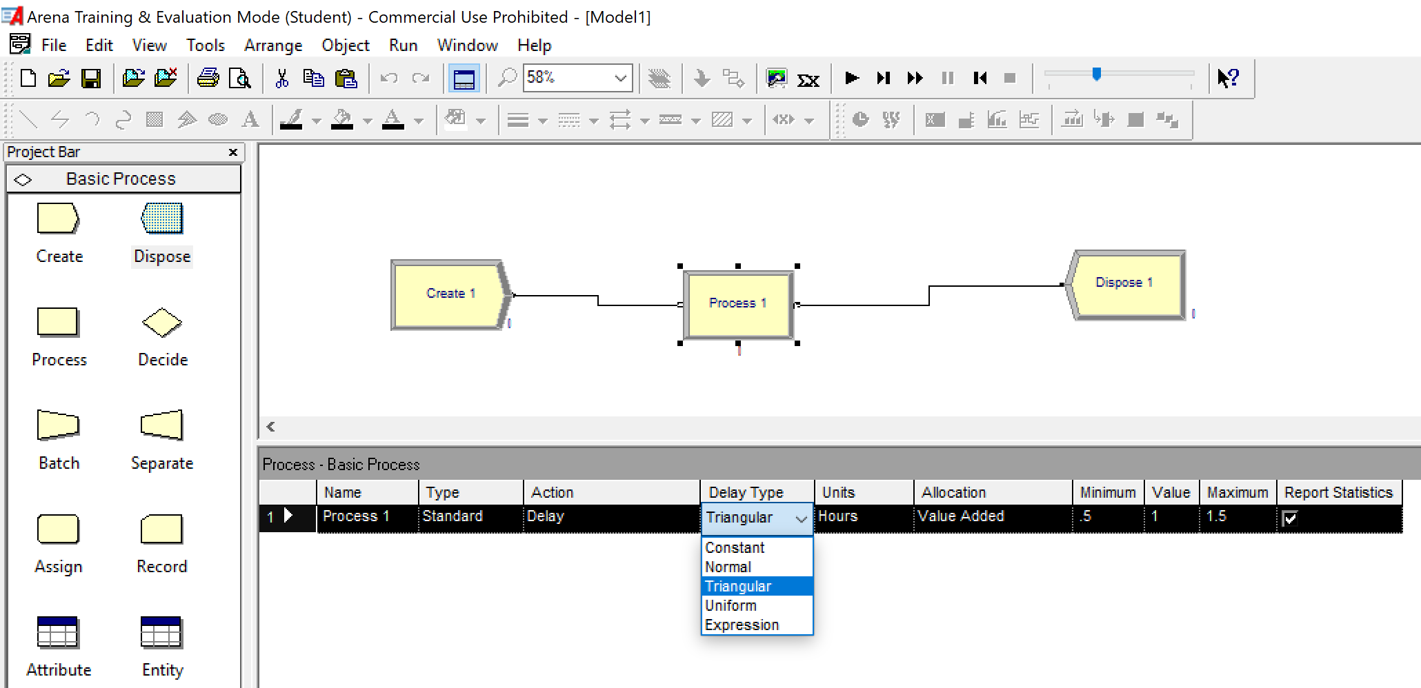
Figure 2:An impression of a simple model in the Arena DES tool.

References¶

Koole, G. (2019). An Introduction to Business Analytics. Chapter 5, “Simulation.”
Kristiansen, O.S., Sandberg, U., Hansen, C., Jensen, M.S., Friederich, J., & Lazarova-Molnar, S. (2022). Experimental comparison of open source discrete-event simulation frameworks. In D. Jiang & H. Song (Eds.), Simulation Tools and Techniques. SIMUtools 2021 (Lecture Notes of the Institute for Computer Sciences, Social Informatics and Telecommunications Engineering, vol. 424). Springer, Cham. Kristiansen et al. (2022)

References¶

Kristiansen, O. S., Sandberg, U., Hansen, C., Jensen, M. S., Friederich, J., & Lazarova-Molnar, S. (2022). Experimental Comparison of Open Source Discrete-Event Simulation Frameworks. In Simulation Tools and Techniques (pp. 315–330). Springer International Publishing. 10.1007/978-3-030-97124-3_24